


Introduction
Aging is a complex process that involves multiple systems, leading to physiological dysregulation, health deterioration, and eventually death. Changes that occur at the molecular and cellular levels as individuals grow older propagate to changes detectable in laboratory tests of blood or other tissues and observable in measurements of various physiological variables in an individual at different ages. Cross-sectional measurements of such biomarkers correspond to the instantaneous profile of the current physiological state of an organism which provides valuable information about the current aging status of the body. Numerous studies show that such biomarkers are associated with risks of death and aging-related diseases (see, e.g., reviews in [1–3]). However, such “snapshots” of the physiological state do not help in understanding how exactly the organism arrived at this particular state. For example, if a person at some age has values of biomarkers that are associated with higher survival chances or reduced risks of diseases (e.g., lower values), it is unclear from the cross-sectional information alone if such outcome is due to lower values of respective biomarkers early in life, or due to their slower change with age, or both. Different studies have shown that dynamic characteristics of individual trajectories of biomarkers are associated with mortality risk and other aging-related traits [4]. To investigate such associations, one needs repeated measurements of biomarkers along with relevant time-to-event outcomes (e.g., mortality, onset of diseases) and other relevant health-related outcomes. Such information is routinely collected in contemporary longitudinal studies on humans and many of those, in addition, contain extensive genetic (and, most recently, various omics) data providing opportunities to explore this additional dimension in relation to aging, health, and longevity.
Analyses of longitudinal studies of aging present special methodological challenges due to inherent complexities that need to be taken into account to avoid biased inference. An essential assumption of such analyses is that the longitudinal outcomes (e.g., biomarkers) can be related to the risk of death so that the probability of having a missing value because of death depends on an unobserved value, which is missing not at random (MNAR) [5]. This means that standard methods such as mixed-effects models [6] or generalized estimating equations [7] are not appropriate in such applications because they assume the data are missing (completely) at random. Ignoring this can lead to severe bias, as is well-known in the statistical literature [8]. Furthermore, biomarkers are subject to measurement error and random biological variability; they can be collected at intermittent sparse examination visits, and typically they are not observed at event times. Ignoring measurement errors or biological variation and using the observed “raw” values of such variables as time-dependent covariates in the Cox regression model may lead to biased estimates and incorrect inferences [9, 10], especially when biomarkers are measured at sparse examinations or with a long time interval before an outcome event. Despite such evidence and well recognized needs for using appropriate methods in analyses of longitudinal data on aging [11–14], the adoption of such methods is slow.
In this paper, we apply one such method developed for dealing with MNAR situations, joint models (JM) [15, 16], to data on mortality and available longitudinal measurements of multiple biomarkers from two visits in the Long Life Family Study (LLFS). We apply the statistical (Mahalanobis) distance measure (denoted as DM) [17] to reduce a high-dimensional biomarker space into a single measure that summarizes information about deviations of biomarkers from an optimal “baseline” state defined in a “reference population” and that is interpreted as the measure of physiological dysregulation [17]. DM trajectories were shown to be good predictors of mortality, frailty, and chronic diseases in different studies [18–21] (with higher DM values associated with higher mortality risk, etc.). The dynamic characteristics of DM trajectories are related to different hidden mechanisms of aging-related changes that produce an increase in the risk of death with age [22], onset of unhealthy lifespan, and survival following the onset of unhealthy lifespan [23]. The LLFS collected follow-up data on mortality and measurements of multiple biomarkers in two visits as well as extensive data on common single nucleotide polymorphisms (SNPs) for genotyped participants. Such information allows one to construct DM using biomarker data from both visits, to explore its dynamics in relation to mortality, and to perform genome-wide association studies (GWAS) to investigate genetic factors associated with such dynamics. However, the methodological complexities indicated above are applicable to this analysis. First, DM is constructed from biomarkers that can have measurement errors and random biological variability and thus appropriate modelling (e.g., joint models [15, 16]) should be used rather than analyses using the observed “raw” values of DM as time-dependent covariates in the Cox model [9, 10]. Second, the LLFS currently has only two visits (at which the biomarkers were collected) and many individuals died before visit 2; thus they will have DM measured only at visit 1. DM is known to be strongly associated with the risk of death [17, 18, 20, 22, 23]. Hence, individuals with adverse dynamics of DM should tend to drop-out earlier due to death (see hypothetical illustration in Figure 1), i.e., the probability of drop-out can depend on missing (unobserved) values of DM. Also, a single observation at visit 1 does not provide information on the future dynamics of DM. However, information on time to death combined with available observations of DM can still be used to infer the dynamics of DM (if modeled appropriately). Here we illustrate this using such modelling (joint models) and show how the estimates from joint models can be used to perform GWAS to infer associations of SNPs with static and dynamic characteristics of the measure of physiological dysregulation (DM).
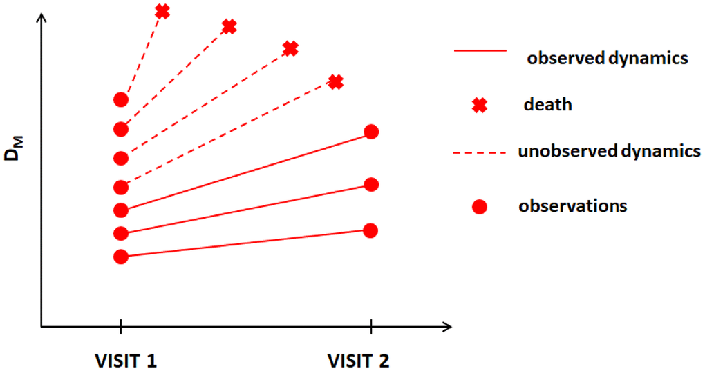
Figure 1. Hypothetical dynamics of the measure of physiological dysregulation (DM) in LLFS among those who survived beyond visit 2 and those who died before visit 2.
Results
Empirical analyses and applications of joint models
Table 1 shows the characteristics of the LLFS sample (for the probands’ and offspring generations and the total sample) including information on variables used in fitting the joint models (see section Specification of joint models). Information on time-dependent variables is presented for each visit. Information on time-independent variables is given for each individual participating in the study (whether he/she was enrolled at baseline or at follow-up visit). See Notes under the table for the number of missing values for each variable.
Table 1. Characteristics of the LLFS Probands and Offspring generations and the total sample.
| Probands | Offspring | Total Sample | |||||||||||||||||||||||||||||||||||||||||||||||||||||||||||||||||||||||||||||||||||||||||||||||||
| Number of participants at in-person visit 1 | 1673 | 3226 | 4899 | ||||||||||||||||||||||||||||||||||||||||||||||||||||||||||||||||||||||||||||||||||||||||||||||||
| Number of visit 1 participants who died before in-person visit 2 | 1050 | 189 | 1239 | ||||||||||||||||||||||||||||||||||||||||||||||||||||||||||||||||||||||||||||||||||||||||||||||||
| Number of visit 1 participants who returned for in-person visit 2 | 554 | 2623 | 3177 | ||||||||||||||||||||||||||||||||||||||||||||||||||||||||||||||||||||||||||||||||||||||||||||||||
| Number of new participants enrolled for in-person visit 2 | 14 | 123 | 137 | ||||||||||||||||||||||||||||||||||||||||||||||||||||||||||||||||||||||||||||||||||||||||||||||||
| Number of participants (returning and new) at in-person visit 2 | 568 | 2746 | 3314 | ||||||||||||||||||||||||||||||||||||||||||||||||||||||||||||||||||||||||||||||||||||||||||||||||
| Number of participants who died after in-person visit 2 | 173 | 43 | 216 | ||||||||||||||||||||||||||||||||||||||||||||||||||||||||||||||||||||||||||||||||||||||||||||||||
| Total number of participants in the study | 1687 | 3349 | 5036 | ||||||||||||||||||||||||||||||||||||||||||||||||||||||||||||||||||||||||||||||||||||||||||||||||
| Number of deaths during the entire follow-up | 1223 | 232 | 1455 | ||||||||||||||||||||||||||||||||||||||||||||||||||||||||||||||||||||||||||||||||||||||||||||||||
| Years from visit 1 to visit 2 (mean ± SD [range]) (for those with both visits) | 7.13 ± 1.02 [5–11] | 8.03 ± 1.1 [5–11] | 7.88 ± 1.13 [5–11] | ||||||||||||||||||||||||||||||||||||||||||||||||||||||||||||||||||||||||||||||||||||||||||||||||
| Age at visit 1 (mean ± SD [range]) | 89.57 ± 6.81 [49–110] | 60.65 ± 8.37 [24–88] | 70.53 ± 15.81 [24–110] | ||||||||||||||||||||||||||||||||||||||||||||||||||||||||||||||||||||||||||||||||||||||||||||||||
| Age at visit 2 (mean ± SD [range]) | 92.93 ± 6.82 [56–110] | 68.4 ± 7.84 [40–95] | 72.39 ± 11.88 [40–110] | ||||||||||||||||||||||||||||||||||||||||||||||||||||||||||||||||||||||||||||||||||||||||||||||||
| Females (%) | 55.78 | 55.03 | 55.28 | ||||||||||||||||||||||||||||||||||||||||||||||||||||||||||||||||||||||||||||||||||||||||||||||||
| Participants from US field centers (%) | 84.77 | 70.02 | 74.96 | ||||||||||||||||||||||||||||||||||||||||||||||||||||||||||||||||||||||||||||||||||||||||||||||||
| Low educated participants (below high school) (%) | 24.72 | 6.42 | 12.55 | ||||||||||||||||||||||||||||||||||||||||||||||||||||||||||||||||||||||||||||||||||||||||||||||||
| Smokers (smoked >100 cigarettes in lifetime) (%) | 37.7 | 45.6 | 42.95 | ||||||||||||||||||||||||||||||||||||||||||||||||||||||||||||||||||||||||||||||||||||||||||||||||
| Medication use at visit 1: anti-diabetic (%) | 7.11 | 4.68 | 5.51 | ||||||||||||||||||||||||||||||||||||||||||||||||||||||||||||||||||||||||||||||||||||||||||||||||
| Medication use at visit 1: anti-hypertensive (%) | 67.54 | 31.43 | 43.76 | ||||||||||||||||||||||||||||||||||||||||||||||||||||||||||||||||||||||||||||||||||||||||||||||||
| Medication use at visit 1: lipid-lowering (%) | 31.68 | 25.33 | 27.5 | ||||||||||||||||||||||||||||||||||||||||||||||||||||||||||||||||||||||||||||||||||||||||||||||||
| Medication use at visit 2: anti-diabetic (%) | 5.28 | 6.08 | 5.94 | ||||||||||||||||||||||||||||||||||||||||||||||||||||||||||||||||||||||||||||||||||||||||||||||||
| Medication use at visit 2: anti-hypertensive (%) | 54.58 | 35.4 | 38.68 | ||||||||||||||||||||||||||||||||||||||||||||||||||||||||||||||||||||||||||||||||||||||||||||||||
| Medication use at visit 2: lipid-lowering (%) | 33.27 | 29.53 | 30.18 | ||||||||||||||||||||||||||||||||||||||||||||||||||||||||||||||||||||||||||||||||||||||||||||||||
| Fasting (>=8 hrs.) at visit 1 (%) | 88.11 | 89.77 | 89.2 | ||||||||||||||||||||||||||||||||||||||||||||||||||||||||||||||||||||||||||||||||||||||||||||||||
| Fasting (>=8 hrs.) at visit 2 (%) | 54.05 | 74.25 | 70.79 | ||||||||||||||||||||||||||||||||||||||||||||||||||||||||||||||||||||||||||||||||||||||||||||||||
| Follow-up period (mean ± SD [range]) | 5.66 ± 2.97 [0–11.9] | 8.36 ± 2.49 [0–12] | 7.46 ± 2.95 [0–12] | ||||||||||||||||||||||||||||||||||||||||||||||||||||||||||||||||||||||||||||||||||||||||||||||||
| Prevalence of cancer, number (%) | 588 (34.85) | 621 (18.54) | 1209 (24.01) | ||||||||||||||||||||||||||||||||||||||||||||||||||||||||||||||||||||||||||||||||||||||||||||||||
| Prevalence of CVD, number (%) | 461 (27.33) | 206 (6.15) | 667 (13.24) | ||||||||||||||||||||||||||||||||||||||||||||||||||||||||||||||||||||||||||||||||||||||||||||||||
| Prevalence of AD or dementia, number (%) | 119 (7.05) | 8 (0.24) | 127 (2.52) | ||||||||||||||||||||||||||||||||||||||||||||||||||||||||||||||||||||||||||||||||||||||||||||||||
| Prevalence of diabetes, number (%) | 162 (9.60) | 212 (6.33) | 374 (7.43) | ||||||||||||||||||||||||||||||||||||||||||||||||||||||||||||||||||||||||||||||||||||||||||||||||
| Incidence of cancer, number (%) | 183 (10.85) | 339 (10.12) | 522 (10.37) | ||||||||||||||||||||||||||||||||||||||||||||||||||||||||||||||||||||||||||||||||||||||||||||||||
| Incidence of CVD, number (%) | 341 (20.21) | 188 (5.61) | 529 (10.50) | ||||||||||||||||||||||||||||||||||||||||||||||||||||||||||||||||||||||||||||||||||||||||||||||||
| Incidence of AD or dementia, number (%) | 119 (7.05) | 27 (0.81) | 146 (2.90) | ||||||||||||||||||||||||||||||||||||||||||||||||||||||||||||||||||||||||||||||||||||||||||||||||
| Incidence of diabetes, number (%) | 23 (1.36) | 112 (3.34) | 135 (2.68) | ||||||||||||||||||||||||||||||||||||||||||||||||||||||||||||||||||||||||||||||||||||||||||||||||
| Note: Number of missing data (Probands, Offspring, Total Sample): indicator of death/lifespan - (0, 0, 0); age at visit 1 - (0, 0, 0); age at visit 2 - (100, 338, 438); sex - (0, 0, 0); country - (0, 0, 0); education - (8, 3, 11); smoking - (6, 14, 20); anti-diabetic drugs at visit 1 - (62, 424, 486); anti-diabetic drugs at visit 2 - (123, 529, 652); anti-hypertensive drugs at visit 1 - (62, 424, 486); anti-hypertensive drugs at visit 2 - (123, 529, 652); lipid-lowering drugs at visit 1 - (62, 424, 486); lipid-lowering drugs at visit 2 - (123, 529, 652); fasting at visit 1 - (3, 16, 19); fasting at visit 2 - (0, 0, 0); follow-up period - (0, 0, 0); cancer - (1, 3, 4); CVD - (1, 3, 4); AD - (5, 3, 8); diabetes - (4, 5, 9) | |||||||||||||||||||||||||||||||||||||||||||||||||||||||||||||||||||||||||||||||||||||||||||||||||||
Table 1 also includes information on prevalent (existing before the baseline visit) and incident (new cases reported after the baseline visit) cases of major aging-related diseases in the LLFS. It shows that participants from the probands’ generation had higher prevalence of major diseases compared to the younger (offspring) generation, as expected. However, for incidence the pattern is not uniform: the proportions of new cancer cases are almost the same in two generations and the proportions of new diabetes cases tended to be higher in the offspring generation. We note also that verified information on causes of deaths of LLFS participants was not available for this study. Therefore, the numbers and proportions of individuals dying from different causes were not determined in this sample.
We constructed the measure of physiological dysregulation (denoted as
Table 2. Biomarkers used in construction of statistical distance measures (DM).
| Name (Unit of Measurement) | Number of Observations Visit 1 | Number of Observations Visit 2 | Number of Observations Total | ||||||||||||||||||||||||||||||||||||||||||||||||||||||||||||||||||||||||||||||||||||||||||||||||
| Absolute monocyte count (10e9/L) | 4,495 | 2,252 | 6,747 | ||||||||||||||||||||||||||||||||||||||||||||||||||||||||||||||||||||||||||||||||||||||||||||||||
| Creatinine (mg/dL) | 4,658 | 2,615 | 7,273 | ||||||||||||||||||||||||||||||||||||||||||||||||||||||||||||||||||||||||||||||||||||||||||||||||
| Diastolic blood pressure (mmHg) | 4,757 | 2,777 | 7,534 | ||||||||||||||||||||||||||||||||||||||||||||||||||||||||||||||||||||||||||||||||||||||||||||||||
| Forced vital capacity (mL) | 4,399 | 2,353 | 6,752 | ||||||||||||||||||||||||||||||||||||||||||||||||||||||||||||||||||||||||||||||||||||||||||||||||
| Grip strength (kg) | 4,731 | 2,714 | 7,445 | ||||||||||||||||||||||||||||||||||||||||||||||||||||||||||||||||||||||||||||||||||||||||||||||||
| Hematocrit (%) | 4,522 | 2,571 | 7,093 | ||||||||||||||||||||||||||||||||||||||||||||||||||||||||||||||||||||||||||||||||||||||||||||||||
| Glycosylated hemoglobin (%) | 4,626 | 2,596 | 7,222 | ||||||||||||||||||||||||||||||||||||||||||||||||||||||||||||||||||||||||||||||||||||||||||||||||
| Mean corpuscular volume (fl) | 4,519 | 2,569 | 7,088 | ||||||||||||||||||||||||||||||||||||||||||||||||||||||||||||||||||||||||||||||||||||||||||||||||
| Pulse pressure (mmHg) | 4,757 | 2,777 | 7,534 | ||||||||||||||||||||||||||||||||||||||||||||||||||||||||||||||||||||||||||||||||||||||||||||||||
| Red cell distribution width (%) | 4,506 | 2,569 | 7,075 | ||||||||||||||||||||||||||||||||||||||||||||||||||||||||||||||||||||||||||||||||||||||||||||||||
| Total cholesterol (mg/dL) | 4,658 | 2,613 | 7,271 | ||||||||||||||||||||||||||||||||||||||||||||||||||||||||||||||||||||||||||||||||||||||||||||||||
| White blood cell count (10e9/L) | 4,521 | 2,555 | 7,076 | ||||||||||||||||||||||||||||||||||||||||||||||||||||||||||||||||||||||||||||||||||||||||||||||||
| Note: Biomarkers included in | |||||||||||||||||||||||||||||||||||||||||||||||||||||||||||||||||||||||||||||||||||||||||||||||||||
We compared the average values of DM at visit 1 between (1) those who died between visit 1 and visit 2 and (2) those who survived beyond visit 2. The average values of DM at visit 1 for those who died were significantly higher than those for the second group (see Table 3). Similar patterns were observed when stratified by sex, with larger and more significant differences for the “original” DM variants. These analyses indicate that the situation depicted in Figure 1 is likely to be happening here, i.e., participants with higher values of DM and/or higher rates of change tend to die earlier thus creating the paradigm for application of appropriate statistical techniques for joint analyses of longitudinal observations of DM and time-to-event data on mortality.
Table 3. Average values of DM at visit 1 among those who died between visit 1 and visit 2 and those who survived beyond visit 2 (standard deviations in parentheses).
| DM | Total Sample | Females | Males | ||||||
| Died before Visit 2 | Alive at Visit 2 | P-value | Died before Visit 2 | Alive at Visit 2 | P-value | Died before Visit 2 | Alive at Visit 2 | P-value | |
| 1.58 (0.42) | 0.90 (0.48) | 2.1×10-254 | 1.55 (0.42) | 0.89 (0.47) | 2.3×10-116 | 1.62 (0.42) | 0.91 (0.50) | 5.1×10-138 | |
| 1.34 (0.40) | 0.97 (0.41) | 1.7×10-125 | 1.38 (0.38) | 0.98 (0.41) | 8.3×10-80 | 1.31 (0.42) | 0.97 (0.40) | 3.1×10-51 | |
| 1.51 (0.21) | 1.15 (0.25) | 3.4×10-257 | 1.51 (0.21) | 1.15 (0.25) | 1.6×10-133 | 1.50 (0.22) | 1.16 (0.25) | 4.1×10-124 | |
| 0.87 (0.49) | 0.81 (0.47) | 4.8×10⁻⁴ | 0.87 (0.50) | 0.82 (0.47) | 0.084 | 0.88 (0.47) | 0.79 (0.47) | 8.5×10⁻⁴ | |
| 0.92 (0.41) | 0.85 (0.37) | 5.7×10⁻⁶ | 0.93 (0.40) | 0.85 (0.38) | 4.6×10⁻⁵ | 0.90 (0.41) | 0.86 (0.37) | 0.018 | |
| 1.14 (0.24) | 1.09 (0.23) | 3.2×10⁻⁸ | 1.15 (0.24) | 1.09 (0.24) | 1.4×10⁻⁵ | 1.14 (0.24) | 1.09 (0.22) | 4.5×10⁻⁴ | |
Table 4 shows the results of application of the joint models to DM variants
Table 4. Results of the joint models applied to DM variants
| DM | Variable | Longitudinal | Survival | ||||||||||||||||||||||||||||||||||||||||||||||||||||||||||||||||||||||||||||||||||||||||||||||||
| Coef. | 95% CI | P-value | Coef. | HR | 95 % CI | P-value | |||||||||||||||||||||||||||||||||||||||||||||||||||||||||||||||||||||||||||||||||||||||||||||
| DM | 1.380 | 2.10 | [1.718, 2.577] | 6.6×10⁻¹³ | |||||||||||||||||||||||||||||||||||||||||||||||||||||||||||||||||||||||||||||||||||||||||||||||
| AgeV1 | 0.023 | [0.022, 0.024] | 0 | 0.096 | 1.10 | [1.089, 1.112] | 6.7×10-77 | ||||||||||||||||||||||||||||||||||||||||||||||||||||||||||||||||||||||||||||||||||||||||||||
| SexM | 0.071 | [0.047, 0.095] | 7.9×10⁻⁹ | 0.239 | 1.27 | [1.110, 1.453] | 5.0×10⁻⁴ | ||||||||||||||||||||||||||||||||||||||||||||||||||||||||||||||||||||||||||||||||||||||||||||
| IsDK | -0.117 | [-0.147, -0.088] | 8.9×10⁻¹⁵ | 0.486 | 1.63 | [1.352, 1.954] | 2.3×10⁻⁷ | ||||||||||||||||||||||||||||||||||||||||||||||||||||||||||||||||||||||||||||||||||||||||||||
| LowEduc | 0.063 | [0.021, 0.105] | 0.003 | 0.005 | 1.01 | [0.851, 1.186] | 0.955 | ||||||||||||||||||||||||||||||||||||||||||||||||||||||||||||||||||||||||||||||||||||||||||||
| Smoke100 | 0.026 | [0.002, 0.050] | 0.036 | 0.134 | 1.14 | [1.001, 1.305] | 0.048 | ||||||||||||||||||||||||||||||||||||||||||||||||||||||||||||||||||||||||||||||||||||||||||||
| DrugDiab | 0.144 | [0.097, 0.191] | 2.4×10⁻⁹ | ||||||||||||||||||||||||||||||||||||||||||||||||||||||||||||||||||||||||||||||||||||||||||||||||
| DrugHtn | 0.033 | [0.009, 0.058] | 0.008 | ||||||||||||||||||||||||||||||||||||||||||||||||||||||||||||||||||||||||||||||||||||||||||||||||
| DrugLipid | 0.0003 | [-0.025, 0.026] | 0.983 | ||||||||||||||||||||||||||||||||||||||||||||||||||||||||||||||||||||||||||||||||||||||||||||||||
| Fasting | -0.026 | [-0.065, 0.012] | 0.183 | ||||||||||||||||||||||||||||||||||||||||||||||||||||||||||||||||||||||||||||||||||||||||||||||||
| TimeV1 | 0.017 | [0.014, 0.020] | 2.8×10⁻³⁵ | ||||||||||||||||||||||||||||||||||||||||||||||||||||||||||||||||||||||||||||||||||||||||||||||||
| DM | 1.190 | 1.66 | [1.420, 1.937] | 1.7×10⁻¹⁰ | |||||||||||||||||||||||||||||||||||||||||||||||||||||||||||||||||||||||||||||||||||||||||||||||
| AgeV1 | 0.011 | [0.011, 0.012] | 6×10-177 | 0.109 | 1.12 | [1.107, 1.123] | 4.6×10-200 | ||||||||||||||||||||||||||||||||||||||||||||||||||||||||||||||||||||||||||||||||||||||||||||
| SexM | -0.013 | [-0.034, 0.008] | 0.221 | 0.385 | 1.47 | [1.303, 1.658] | 3.5×10⁻¹⁰ | ||||||||||||||||||||||||||||||||||||||||||||||||||||||||||||||||||||||||||||||||||||||||||||
| IsDK | 0.008 | [-0.018, 0.034] | 0.54 | 0.307 | 1.36 | [1.159, 1.593] | 1.6×10⁻⁴ | ||||||||||||||||||||||||||||||||||||||||||||||||||||||||||||||||||||||||||||||||||||||||||||
| LowEduc | 0.039 | [0.003, 0.074] | 0.034 | 0.024 | 1.02 | [0.881, 1.192] | 0.75 | ||||||||||||||||||||||||||||||||||||||||||||||||||||||||||||||||||||||||||||||||||||||||||||
| Smoke100 | 0.026 | [0.005, 0.047] | 0.017 | 0.110 | 1.12 | [0.989, 1.259] | 0.075 | ||||||||||||||||||||||||||||||||||||||||||||||||||||||||||||||||||||||||||||||||||||||||||||
| DrugDiab | 0.303 | [0.262, 0.344] | 3.6×10-47 | ||||||||||||||||||||||||||||||||||||||||||||||||||||||||||||||||||||||||||||||||||||||||||||||||
| DrugHtn | 0.068 | [0.046, 0.089] | 8.2×10⁻¹⁰ | ||||||||||||||||||||||||||||||||||||||||||||||||||||||||||||||||||||||||||||||||||||||||||||||||
| DrugLipid | -0.018 | [-0.040, 0.004] | 0.116 | ||||||||||||||||||||||||||||||||||||||||||||||||||||||||||||||||||||||||||||||||||||||||||||||||
| Fasting | -0.023 | [-0.057, 0.011] | 0.182 | ||||||||||||||||||||||||||||||||||||||||||||||||||||||||||||||||||||||||||||||||||||||||||||||||
| TimeV1 | 0.019 | [0.016, 0.021] | 4.5×10-57 | ||||||||||||||||||||||||||||||||||||||||||||||||||||||||||||||||||||||||||||||||||||||||||||||||
| DM | 2.883 | 2.22 | [1.841, 2.673] | 5.8×10⁻¹⁷ | |||||||||||||||||||||||||||||||||||||||||||||||||||||||||||||||||||||||||||||||||||||||||||||||
| AgeV1 | 0.011 | [0.011, 0.012] | 0 | 0.090 | 1.09 | [1.084, 1.105] | 2.4×10-80 | ||||||||||||||||||||||||||||||||||||||||||||||||||||||||||||||||||||||||||||||||||||||||||||
| SexM | 0.018 | [0.006, 0.031] | 0.005 | 0.317 | 1.37 | [1.203, 1.568] | 2.7×10⁻⁶ | ||||||||||||||||||||||||||||||||||||||||||||||||||||||||||||||||||||||||||||||||||||||||||||
| IsDK | -0.027 | [-0.042, -0.011] | 6.2×10⁻⁴ | 0.373 | 1.45 | [1.212, 1.739] | 5.1×10⁻⁵ | ||||||||||||||||||||||||||||||||||||||||||||||||||||||||||||||||||||||||||||||||||||||||||||
| LowEduc | 0.042 | [0.021, 0.064] | 1.3×10⁻⁴ | 0.028 | 1.03 | [0.870, 1.217] | 0.741 | ||||||||||||||||||||||||||||||||||||||||||||||||||||||||||||||||||||||||||||||||||||||||||||
| Smoke100 | 0.018 | [0.005, 0.031] | 0.005 | 0.077 | 1.08 | [0.945, 1.235] | 0.257 | ||||||||||||||||||||||||||||||||||||||||||||||||||||||||||||||||||||||||||||||||||||||||||||
| DrugDiab | 0.160 | [0.136, 0.185] | 3.4×10-37 | ||||||||||||||||||||||||||||||||||||||||||||||||||||||||||||||||||||||||||||||||||||||||||||||||
| DrugHtn | 0.038 | [0.025, 0.051] | 7.1×10⁻⁹ | ||||||||||||||||||||||||||||||||||||||||||||||||||||||||||||||||||||||||||||||||||||||||||||||||
| DrugLipid | -0.001 | [-0.014, 0.012] | 0.922 | ||||||||||||||||||||||||||||||||||||||||||||||||||||||||||||||||||||||||||||||||||||||||||||||||
| Fasting | -0.025 | [-0.045, -0.005] | 0.016 | ||||||||||||||||||||||||||||||||||||||||||||||||||||||||||||||||||||||||||||||||||||||||||||||||
| TimeV1 | 0.014 | [0.012, 0.015] | 7.9×10-81 | ||||||||||||||||||||||||||||||||||||||||||||||||||||||||||||||||||||||||||||||||||||||||||||||||
| Notes: 1.Variables: AgeV1: Age at visit 1, SexM: Sex (1 – male, 0 – female), IsDK: Participant is from Denmark (1) or USA (0), LowEduc: Low education (1 – below high school, 0 – otherwise), Smoke100: Smoker (1 – smoked >100 cigarettes in lifetime, 0 – otherwise), DrugDiab: Takes (1) or does not take (0) anti-diabetic drugs, DrugHtn: Takes (1) or does not take (0) anti-hypertensive drugs, DrugLipid: Takes (1) or does not take (0) lipid-lowering drugs, Fasting: Fasting (1 – >=8 hrs., 0 – otherwise), TimeV1: Follow-up period since visit 1. | |||||||||||||||||||||||||||||||||||||||||||||||||||||||||||||||||||||||||||||||||||||||||||||||||||
| 2.Hazard ratios (HR) of all-cause mortality risk for DM variables are per standard deviation: | |||||||||||||||||||||||||||||||||||||||||||||||||||||||||||||||||||||||||||||||||||||||||||||||||||
For comparison, the results of application of the Cox model to the same data (with the respective DM variant included as a time-dependent covariate carried forward from visit 1 and updated if there is a visit 2) are presented in Table 5. This table shows that the HRs for DM from joint models were 1.3 to 1.4 times larger than the estimates from the Cox model.
Table 5. Results of the Cox model with DM as a time-dependent covariate.
| DM | Variable | Coef. | HR | 95 % CI | P-value | ||||||||||||||||||||||||||||||||||||||||||||||||||||||||||||||||||||||||||||||||||||||||||||||
| DM | 0.877 | 1.60 | [1.460, 1.764] | 1.0×10⁻²² | |||||||||||||||||||||||||||||||||||||||||||||||||||||||||||||||||||||||||||||||||||||||||||||||
| AgeV1 | 0.105 | 1.11 | [1.103, 1.120] | 3.6×10-162 | |||||||||||||||||||||||||||||||||||||||||||||||||||||||||||||||||||||||||||||||||||||||||||||||
| SexM | 0.275 | 1.32 | [1.159, 1.494] | 2.2×10⁻⁵ | |||||||||||||||||||||||||||||||||||||||||||||||||||||||||||||||||||||||||||||||||||||||||||||||
| IsDK | 0.366 | 1.44 | [1.219, 1.705] | 1.9×10⁻⁵ | |||||||||||||||||||||||||||||||||||||||||||||||||||||||||||||||||||||||||||||||||||||||||||||||
| LowEduc | 0.051 | 1.05 | [0.901, 1.230] | 0.517 | |||||||||||||||||||||||||||||||||||||||||||||||||||||||||||||||||||||||||||||||||||||||||||||||
| Smoke100 | 0.131 | 1.14 | [1.005, 1.293] | 0.041 | |||||||||||||||||||||||||||||||||||||||||||||||||||||||||||||||||||||||||||||||||||||||||||||||
| DM | 0.478 | 1.23 | [1.147, 1.309] | 1.8×10⁻⁹ | |||||||||||||||||||||||||||||||||||||||||||||||||||||||||||||||||||||||||||||||||||||||||||||||
| AgeV1 | 0.121 | 1.13 | [1.121, 1.136] | 5.7×10-296 | |||||||||||||||||||||||||||||||||||||||||||||||||||||||||||||||||||||||||||||||||||||||||||||||
| SexM | 0.386 | 1.47 | [1.309, 1.655] | 9.6×10⁻¹¹ | |||||||||||||||||||||||||||||||||||||||||||||||||||||||||||||||||||||||||||||||||||||||||||||||
| IsDK | 0.324 | 1.38 | [1.184, 1.615] | 4.2×10⁻⁵ | |||||||||||||||||||||||||||||||||||||||||||||||||||||||||||||||||||||||||||||||||||||||||||||||
| LowEduc | 0.036 | 1.04 | [0.897, 1.199] | 0.626 | |||||||||||||||||||||||||||||||||||||||||||||||||||||||||||||||||||||||||||||||||||||||||||||||
| Smoke100 | 0.133 | 1.14 | [1.016, 1.285] | 0.026 | |||||||||||||||||||||||||||||||||||||||||||||||||||||||||||||||||||||||||||||||||||||||||||||||
| DM | 1.666 | 1.58 | [1.442, 1.740] | 7.4×10⁻²² | |||||||||||||||||||||||||||||||||||||||||||||||||||||||||||||||||||||||||||||||||||||||||||||||
| AgeV1 | 0.108 | 1.11 | [1.106, 1.123] | 2.7×10-175 | |||||||||||||||||||||||||||||||||||||||||||||||||||||||||||||||||||||||||||||||||||||||||||||||
| SexM | 0.364 | 1.44 | [1.269, 1.634] | 1.7×10⁻⁸ | |||||||||||||||||||||||||||||||||||||||||||||||||||||||||||||||||||||||||||||||||||||||||||||||
| IsDK | 0.360 | 1.43 | [1.211, 1.698] | 2.9×10⁻⁵ | |||||||||||||||||||||||||||||||||||||||||||||||||||||||||||||||||||||||||||||||||||||||||||||||
| LowEduc | 0.055 | 1.06 | [0.904, 1.236] | 0.489 | |||||||||||||||||||||||||||||||||||||||||||||||||||||||||||||||||||||||||||||||||||||||||||||||
| Smoke100 | 0.105 | 1.11 | [0.978, 1.261] | 0.106 | |||||||||||||||||||||||||||||||||||||||||||||||||||||||||||||||||||||||||||||||||||||||||||||||
| Notes: Variables: AgeV1: Age at visit 1, SexM: Sex (1 – male, 0 – female), IsDK: Participant is from Denmark (1) or USA (0), LowEduc: Low education (1 – below high school, 0 – otherwise), Smoke100: Smoker (1 – smoked >100 cigarettes in lifetime, 0 – otherwise). | |||||||||||||||||||||||||||||||||||||||||||||||||||||||||||||||||||||||||||||||||||||||||||||||||||
| Hazard ratios (HR) of all-cause mortality risk for DM variables are per standard deviation: | |||||||||||||||||||||||||||||||||||||||||||||||||||||||||||||||||||||||||||||||||||||||||||||||||||
The results for the “age-dependent” DM variants (
Table 6. Results of the joint models applied to age-dependent DM variants
| DM | Variable | Longitudinal | Survival | ||||||||||||||||||||||||||||||||||||||||||||||||||||||||||||||||||||||||||||||||||||||||||||||||
| Coef. | 95% CI | P-value | Coef. | HR | 95 % CI | P-value | |||||||||||||||||||||||||||||||||||||||||||||||||||||||||||||||||||||||||||||||||||||||||||||
| DM | 0.562 | 1.31 | [1.155, 1.476] | 2.1×10⁻⁵ | |||||||||||||||||||||||||||||||||||||||||||||||||||||||||||||||||||||||||||||||||||||||||||||||
| AgeV1 | 0.00006 | [-0.001, 0.001] | 0.904 | 0.125 | 1.13 | [1.125, 1.140] | 9.1×10-300 | ||||||||||||||||||||||||||||||||||||||||||||||||||||||||||||||||||||||||||||||||||||||||||||
| SexM | 0.003 | [-0.024, 0.030] | 0.821 | 0.364 | 1.44 | [1.268, 1.634] | 1.9×10⁻⁸ | ||||||||||||||||||||||||||||||||||||||||||||||||||||||||||||||||||||||||||||||||||||||||||||
| IsDK | 0.045 | [0.012, 0.079] | 0.008 | 0.255 | 1.29 | [1.089, 1.530] | 0.003 | ||||||||||||||||||||||||||||||||||||||||||||||||||||||||||||||||||||||||||||||||||||||||||||
| LowEduc | 0.030 | [-0.018, 0.077] | 0.221 | 0.066 | 1.07 | [0.912, 1.251] | 0.413 | ||||||||||||||||||||||||||||||||||||||||||||||||||||||||||||||||||||||||||||||||||||||||||||
| Smoke100 | 0.037 | [0.010, 0.065] | 0.007 | 0.129 | 1.14 | [1.000, 1.292] | 0.049 | ||||||||||||||||||||||||||||||||||||||||||||||||||||||||||||||||||||||||||||||||||||||||||||
| DrugDiab | 0.100 | [0.046, 0.154] | 2.7×10⁻⁸ | ||||||||||||||||||||||||||||||||||||||||||||||||||||||||||||||||||||||||||||||||||||||||||||||||
| DrugHtn | 0.011 | [-0.017, 0.04] | 0.427 | ||||||||||||||||||||||||||||||||||||||||||||||||||||||||||||||||||||||||||||||||||||||||||||||||
| DrugLipid | 0.017 | [-0.012, 0.046] | 0.247 | ||||||||||||||||||||||||||||||||||||||||||||||||||||||||||||||||||||||||||||||||||||||||||||||||
| Fasting | -0.011 | [-0.055, 0.033] | 0.623 | ||||||||||||||||||||||||||||||||||||||||||||||||||||||||||||||||||||||||||||||||||||||||||||||||
| TimeV1 | -0.003 | [-0.006, -0.0003] | 0.032 | ||||||||||||||||||||||||||||||||||||||||||||||||||||||||||||||||||||||||||||||||||||||||||||||||
| DM | 1.332 | 1.67 | [1.419, 1.965] | 6.6×10⁻¹⁰ | |||||||||||||||||||||||||||||||||||||||||||||||||||||||||||||||||||||||||||||||||||||||||||||||
| AgeV1 | -0.0008 | [-0.001, -0.0004] | 0.040 | 0.127 | 1.14 | [1.129, 1.143] | 0 | ||||||||||||||||||||||||||||||||||||||||||||||||||||||||||||||||||||||||||||||||||||||||||||
| SexM | -0.0008 | [-0.021, 0.020] | 0.939 | 0.376 | 1.46 | [1.290, 1.644] | 1.3×10⁻⁹ | ||||||||||||||||||||||||||||||||||||||||||||||||||||||||||||||||||||||||||||||||||||||||||||
| IsDK | 0.013 | [-0.013, 0.038] | 0.325 | 0.282 | 1.33 | [1.129, 1.556] | 5.7×10⁻⁴ | ||||||||||||||||||||||||||||||||||||||||||||||||||||||||||||||||||||||||||||||||||||||||||||
| LowEduc | 0.041 | [0.006, 0.077] | 0.022 | -0.001 | .998 | [0.856, 1.165] | 0.986 | ||||||||||||||||||||||||||||||||||||||||||||||||||||||||||||||||||||||||||||||||||||||||||||
| Smoke100 | 0.024 | [0.003, 0.045] | 0.024 | 0.112 | 1.12 | [0.989, 1.263] | 0.074 | ||||||||||||||||||||||||||||||||||||||||||||||||||||||||||||||||||||||||||||||||||||||||||||
| DrugDiab | 0.288 | [0.247, 0.330] | 8.1×10-43 | ||||||||||||||||||||||||||||||||||||||||||||||||||||||||||||||||||||||||||||||||||||||||||||||||
| DrugHtn | 0.037 | [0.016, 0.059] | 7.3×10⁻⁴ | ||||||||||||||||||||||||||||||||||||||||||||||||||||||||||||||||||||||||||||||||||||||||||||||||
| DrugLipid | -0.033 | [-0.055, -0.010] | 0.004 | ||||||||||||||||||||||||||||||||||||||||||||||||||||||||||||||||||||||||||||||||||||||||||||||||
| Fasting | -0.029 | [-0.063, 0.005] | 0.098 | ||||||||||||||||||||||||||||||||||||||||||||||||||||||||||||||||||||||||||||||||||||||||||||||||
| TimeV1 | -0.001 | [-0.004, 0.001] | 0.321 | ||||||||||||||||||||||||||||||||||||||||||||||||||||||||||||||||||||||||||||||||||||||||||||||||
| DM | 2.246 | 1.70 | [1.445, 2.005] | 1.9×10⁻¹⁰ | |||||||||||||||||||||||||||||||||||||||||||||||||||||||||||||||||||||||||||||||||||||||||||||||
| AgeV1 | -0.0002 | [-0.0007, 0.0003] | 0.420 | 0.128 | 1.14 | [1.129, 1.145] | 4.2×10-279 | ||||||||||||||||||||||||||||||||||||||||||||||||||||||||||||||||||||||||||||||||||||||||||||
| SexM | 0.003 | [-0.011, 0.016] | 0.683 | 0.383 | 1.47 | [1.286, 1.674] | 1.2×10⁻⁸ | ||||||||||||||||||||||||||||||||||||||||||||||||||||||||||||||||||||||||||||||||||||||||||||
| IsDK | 0.010 | [-0.006, 0.027] | 0.223 | 0.279 | 1.32 | [1.109, 1.576] | 0.002 | ||||||||||||||||||||||||||||||||||||||||||||||||||||||||||||||||||||||||||||||||||||||||||||
| LowEduc | 0.030 | [0.006, 0.054] | 0.013 | 0.023 | 1.02 | [0.866, 1.209] | 0.791 | ||||||||||||||||||||||||||||||||||||||||||||||||||||||||||||||||||||||||||||||||||||||||||||
| Smoke100 | 0.023 | [0.01, 0.037] | 7.3×10⁻⁴ | 0.088 | 1.09 | [0.956, 1.247] | 0.196 | ||||||||||||||||||||||||||||||||||||||||||||||||||||||||||||||||||||||||||||||||||||||||||||
| DrugDiab | 0.157 | [0.130, 0.184] | 1.0×10⁻²⁹ | ||||||||||||||||||||||||||||||||||||||||||||||||||||||||||||||||||||||||||||||||||||||||||||||||
| DrugHtn | 0.016 | [0.002, 0.030] | 0.024 | ||||||||||||||||||||||||||||||||||||||||||||||||||||||||||||||||||||||||||||||||||||||||||||||||
| DrugLipid | -0.012 | [-0.026, 0.003] | 0.114 | ||||||||||||||||||||||||||||||||||||||||||||||||||||||||||||||||||||||||||||||||||||||||||||||||
| Fasting | -0.019 | [-0.042, 0.004] | 0.103 | ||||||||||||||||||||||||||||||||||||||||||||||||||||||||||||||||||||||||||||||||||||||||||||||||
| TimeV1 | -0.001 | [-0.003, 0.001] | 0.198 | ||||||||||||||||||||||||||||||||||||||||||||||||||||||||||||||||||||||||||||||||||||||||||||||||
| Notes: Variables: AgeV1: Age at visit 1, SexM: Sex (1 – male, 0 – female), IsDK: Participant is from Denmark (1) or USA (0), LowEduc: Low education (1 – below high school, 0 – otherwise), Smoke100: Smoker (1 – smoked >100 cigarettes in lifetime, 0 – otherwise), DrugDiab: Takes (1) or does not take (0) anti-diabetic drugs, DrugHtn: Takes (1) or does not take (0) anti-hypertensive drugs, DrugLipid: Takes (1) or does not take (0) lipid-lowering drugs, Fasting: Fasting (1 – >=8 hrs., 0 – otherwise), TimeV1: Follow-up period since visit 1. | |||||||||||||||||||||||||||||||||||||||||||||||||||||||||||||||||||||||||||||||||||||||||||||||||||
Table 7. Results of the Cox model with age-dependent DM as a time-dependent covariate.
| DM | Variable | Coef. | HR | 95 % CI | P-value | ||||||||||||||||||||||||||||||||||||||||||||||||||||||||||||||||||||||||||||||||||||||||||||||
| DM | 0.284 | 1.14 | [1.077, 1.216] | 1.2×10⁻⁵ | |||||||||||||||||||||||||||||||||||||||||||||||||||||||||||||||||||||||||||||||||||||||||||||||
| AgeV1 | 0.126 | 1.13 | [1.127, 1.142] | 0.4×10-309 | |||||||||||||||||||||||||||||||||||||||||||||||||||||||||||||||||||||||||||||||||||||||||||||||
| SexM | 0.375 | 1.46 | [1.284, 1.650] | 4.7×10⁻⁹ | |||||||||||||||||||||||||||||||||||||||||||||||||||||||||||||||||||||||||||||||||||||||||||||||
| IsDK | 0.274 | 1.32 | [1.112, 1.556] | 0.001 | |||||||||||||||||||||||||||||||||||||||||||||||||||||||||||||||||||||||||||||||||||||||||||||||
| LowEduc | 0.075 | 1.08 | [0.922, 1.259] | 0.348 | |||||||||||||||||||||||||||||||||||||||||||||||||||||||||||||||||||||||||||||||||||||||||||||||
| Smoke100 | 0.131 | 1.14 | [1.004, 1.293] | 0.043 | |||||||||||||||||||||||||||||||||||||||||||||||||||||||||||||||||||||||||||||||||||||||||||||||
| DM | 0.503 | 1.21 | [1.148, 1.283] | 8.7×10⁻¹² | |||||||||||||||||||||||||||||||||||||||||||||||||||||||||||||||||||||||||||||||||||||||||||||||
| AgeV1 | 0.128 | 1.14 | [1.129, 1.143] | 0 | |||||||||||||||||||||||||||||||||||||||||||||||||||||||||||||||||||||||||||||||||||||||||||||||
| SexM | 0.376 | 1.46 | [1.296, 1.637] | 3.1×10⁻¹⁰ | |||||||||||||||||||||||||||||||||||||||||||||||||||||||||||||||||||||||||||||||||||||||||||||||
| IsDK | 0.301 | 1.35 | [1.158, 1.578] | 1.4×10⁻⁴ | |||||||||||||||||||||||||||||||||||||||||||||||||||||||||||||||||||||||||||||||||||||||||||||||
| LowEduc | 0.024 | 1.02 | [0.885, 1.185] | 0.748 | |||||||||||||||||||||||||||||||||||||||||||||||||||||||||||||||||||||||||||||||||||||||||||||||
| Smoke100 | 0.124 | 1.13 | [1.006, 1.273] | 0.04 | |||||||||||||||||||||||||||||||||||||||||||||||||||||||||||||||||||||||||||||||||||||||||||||||
| DM | 0.938 | 1.25 | [1.173, 1.329] | 3.1×10⁻¹² | |||||||||||||||||||||||||||||||||||||||||||||||||||||||||||||||||||||||||||||||||||||||||||||||
| AgeV1 | 0.128 | 1.14 | [1.129, 1.144] | 0.6×10-309 | |||||||||||||||||||||||||||||||||||||||||||||||||||||||||||||||||||||||||||||||||||||||||||||||
| SexM | 0.395 | 1.48 | [1.307, 1.685] | 1.1×10⁻⁹ | |||||||||||||||||||||||||||||||||||||||||||||||||||||||||||||||||||||||||||||||||||||||||||||||
| IsDK | 0.284 | 1.33 | [1.123, 1.572] | 9.2×10⁻⁴ | |||||||||||||||||||||||||||||||||||||||||||||||||||||||||||||||||||||||||||||||||||||||||||||||
| LowEduc | 0.067 | 1.07 | [0.914, 1.252] | 0.402 | |||||||||||||||||||||||||||||||||||||||||||||||||||||||||||||||||||||||||||||||||||||||||||||||
| Smoke100 | 0.100 | 1.11 | [0.973, 1.255] | 0.124 | |||||||||||||||||||||||||||||||||||||||||||||||||||||||||||||||||||||||||||||||||||||||||||||||
| Notes: Variables: AgeV1: Age at visit 1, SexM: Sex (1 – male, 0 – female), IsDK: Participant is from Denmark (1) or USA (0), LowEduc: Low education (1 – below high school, 0 – otherwise), Smoke100: Smoker (1 – smoked >100 cigarettes in lifetime, 0 – otherwise). Hazard ratios (HR) of all-cause mortality risk for DM variables are per standard deviation: | |||||||||||||||||||||||||||||||||||||||||||||||||||||||||||||||||||||||||||||||||||||||||||||||||||
Genetic analyses of DM-related traits
The R-package JM provides estimates of two types of random effects (random intercept, DM-RI, and random slope, DM-RS) for each individual in the analytic sample; these random effects are the traits used in the genetic analyses (see Methods). Figure 2 presents the results of the GWAS of
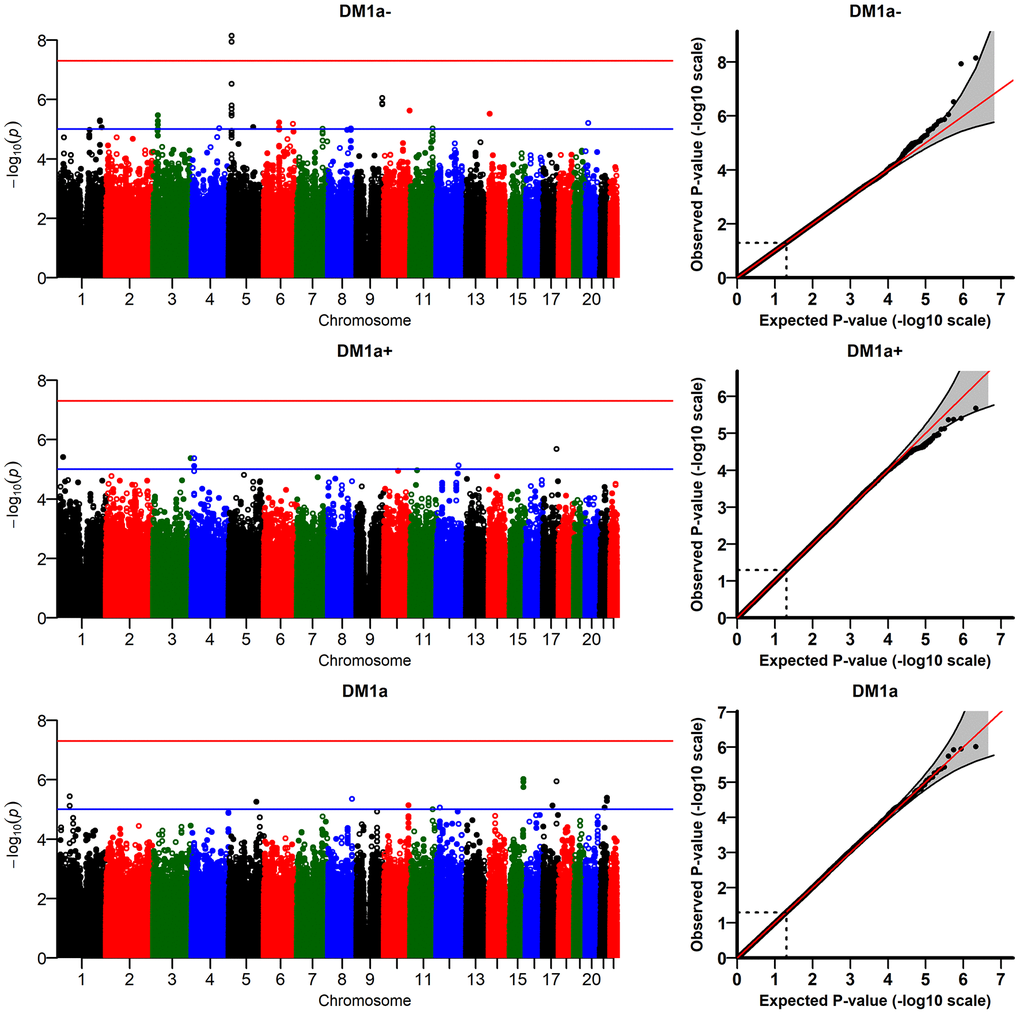
Figure 2. Results of genome-wide association study of random slopes of DM (DM-RS) for “age-dependent” DM variants (
The DM variants were constructed using several biomarkers (see Methods). To check whether the signals observed in the analyses of
We also performed sensitivity analyses running the models with different numbers of principal components (PCs: 1, 2, 5, 10). The top two signals for
(Supplementary Figure 4) did not reach the genome-wide significant level in some models with different numbers of PCs (e.g., p=8.8×10⁻⁸ for the model with 2 PCs). In addition, we performed analyses of DM variants constructed using different sets of biomarkers selected according to other thresholds for correlation with age (absolute value of the correlation ≥ 0.1 and ≥ 0.2) which did not produce any genome-wide significant signals. We also ran the model with time-interaction terms for all covariates (except age) in the fixed effects part of the longitudinal sub-model in JM. All interactions were non-significant except that for country (estimate: -0.008; p = 0.03). The GWAS results for
Discussion
Applications of joint models to composite measures of physiological dysregulation (DM) and genetic analyses of individual characteristics of DM, in the context of research on aging
In this work, we constructed the statistical (Mahalanobis) distance measure (DM) using multiple biomarkers collected at two visits in the LLFS using the original approach from [17] and its “age-dependent” modification that considers deviations of biomarker values from those typical of age peers rather than those of younger individuals. Analyses of longitudinal trajectories of such measures present methodological challenges (see Introduction) that require applying appropriate statistical methodology for correct inference. Here we applied one such method, joint models, for joint analyses of longitudinal observations of DM and follow-up data on mortality for LLFS participants. Applications confirmed that, as in other studies [17, 18, 20, 22, 23], the association of DM with mortality in LLFS is significant and effect sizes are substantial (with larger HRs for the “original” DM variants). Comparisons of joint models with the Cox regression model with DM considered as a time-dependent covariate indicated that the values of the association parameter for DM in the hazard are underestimated in the Cox model, as expected [9, 10, 15]. Even though both models reveal the same direction of the influence and the result remains highly significant so that one may argue that the interpretation of the results in this case is the same in these two approaches, application of an inappropriate approach can still have substantial consequences if, for example, one needs to build a predictive model based on these results. As shown in many studies [4], including our applications to LLFS [24] and other data [23], inclusion of composite measures improves the predictive accuracy of the models for mortality and other health-related outcomes. Therefore, such predictive models should be based on an appropriate statistical approach such as joint models, which effectively account for informative missingness (death), and thus are able to correct for that type of bias.
Joint models is an active area of research in statistics with numerous extensions of the basic model (analyzed in this paper) suggested in the literature that cover a wide range of research applications such as latent classes, competing risks, multivariate models, non-linear models, dynamic predictions, stochastic processes, etc. (see books [15, 16] and recent review papers and tutorials [25–33]). Such extended models can be applied to analyze dynamic characteristics of composite measures such as DM with various outcomes in more comprehensive ways.
One particular approach for joint analyses of longitudinal and time-to-event outcomes, the stochastic process model, SPM (see non-technical introduction in [4] and technical reviews in [34, 35]), is especially relevant in the context of research on aging as the model has components that permit clear biological interpretation in terms of fundamental features of aging-related changes in an organism. Our recent applications [22, 23] of SPM to DM confirmed its significant association with mortality and proxy measures of physiological robustness and resilience, and revealed significant relationships of physiological dysregulation with other hidden aging-related characteristics, such as decline in stress resistance and adaptive capacity which typically are not observed in the data and thus can be analyzed only indirectly through such an analytic approach. The availability of genetic data in longitudinal studies makes it possible to explore genetic determinants of biological aging of individuals based on the dynamics of such composite measures as DM. However, this is still a largely unexplored area. The “genetic” SPM [36–38] allows investigation of genetic determinants of such aging-related characteristics in applications to longitudinal observations of composite biomarkers (such as DM). In particular, recent developments in the SPM methodology [39] have considerably enhanced the computational speed (which was a critical barrier in implementing this approach to large-scale genetic analyses) and opened new avenues for applying this model to GWAS, with far reaching implications for significantly improving our understanding of the genetic underpinnings of complex aging-related traits.
Interpretation of genetic associations with DM: Biological and health effects of genes associated with the increase in physiological dysregulation with age
Table 8 shows the five genes (TRIO, FNBP1, PLXNA4, CADM1, and UBE2E2) corresponding to the top SNPs found in the association analysis of the random slope of DM (for the “age-dependent” DM constructed from biomarkers that decline in late life), including the SNP rs12652543 that reached genome-wide level of significance (other three genes shown in Table 8 will be discussed later). Note that multiple SNPs in these five genes were associated with slopes of DM, many of which were in LD with each other (according to LDlink,https://ldlink.nci.nih.gov). We eliminated the redundant SNPs (r2>0.8), so the SNPs shown in Table 8 represent not only themselves but also LD blocks (r2>0.8) of other (not shown) SNPs associated with DM slopes. We then performed in depth review of scientific literature and information provided by the NCBI Gene (https://www.ncbi.nlm.nih.gov/gene/), and found that four of the above five genes have been implemented in cancer, especially in its progression/prognosis. Three of these genes (TRIO, PLXNA4 [Plexin A4] and CADM1 [TSLC1, SynCAM1]) are also involved in axon guidance and growth (Table 8, last column) [40–46].
Table 8. Top-ranked SNPs from GWAS of the random slope of DM, and respective genes (explanation in Discussion).
| SNP | Chr | Position | A1 | A2 | MAF | P-value | Region | Gene | Gene/protein is involved in | ||||||||||||||||||||||||||||||||||||||||||||||||||||||||||||||||||||||||||||||||||||||||||
| rs12652543 | 5 | 14177235 | A | G | 0.18 | 7.2×10⁻⁹ | intron | TRIO | cancer cells migration, invasion, prognosis, axon guidance, | ||||||||||||||||||||||||||||||||||||||||||||||||||||||||||||||||||||||||||||||||||||||||||
| rs32573 | 5 | 14172108 | G | A | 0.20 | 3.0×10⁻⁷ | intron | TRIO | synapse function, neurite outgrowth, neurotransmission, | ||||||||||||||||||||||||||||||||||||||||||||||||||||||||||||||||||||||||||||||||||||||||||
| rs151473 | 5 | 14123313 | T | C | 0.16 | 1.6×10⁻⁶ | 20kb 5' | TRIO | cognition, intellectual disability | ||||||||||||||||||||||||||||||||||||||||||||||||||||||||||||||||||||||||||||||||||||||||||
| rs72757229 | 9 | 132653055 | G | A | 0.04 | 8.9×10⁻⁷ | intron | FNBP1 | high expression in cancer | ||||||||||||||||||||||||||||||||||||||||||||||||||||||||||||||||||||||||||||||||||||||||||
| rs79434268 | 7 | 131853832 | A | G | 0.07 | 9.8×10⁻⁶ | intron | PLXNA4 (Plexin A4) | axon guidance, Parkinson's, AD, tau, cancer progression | ||||||||||||||||||||||||||||||||||||||||||||||||||||||||||||||||||||||||||||||||||||||||||
| rs1892773 | 11 | 115122626 | C | A | 0.21 | 9.6×10⁻⁶ | intron | CADM1 (TSLC1) | synaptic cell adhesion, axon guidance, cancer prognosis | ||||||||||||||||||||||||||||||||||||||||||||||||||||||||||||||||||||||||||||||||||||||||||
| rs11713090 | 3 | 23570654 | T | G | 0.20 | 3.4×10⁻⁶ | intron | UBE2E2 | T2D | ||||||||||||||||||||||||||||||||||||||||||||||||||||||||||||||||||||||||||||||||||||||||||
| rs1436351 | 3 | 104617973 | G | T | 0.25 | 5.1×10⁻⁵ | 5' of | ALCAM (CD166) | cell adhesion, migration, cancer, axon growth, immunoglobulins | ||||||||||||||||||||||||||||||||||||||||||||||||||||||||||||||||||||||||||||||||||||||||||
| rs13097329 | 3 | 1320815 | A | G | 0.45 | 5.9×10⁻⁵ | intron | CNTN6 | cell adhesion, axon connections, intellectual disability | ||||||||||||||||||||||||||||||||||||||||||||||||||||||||||||||||||||||||||||||||||||||||||
| rs1444261 | 2 | 55354466 | C | T | 0.08 | 1.9×10⁻⁵ | intron | RTN4 (Reticulon4) | nerve growth inhibitor, blocks regeneration | ||||||||||||||||||||||||||||||||||||||||||||||||||||||||||||||||||||||||||||||||||||||||||
| Notes: SNP – rs-number; Chr – chromosome number; Position – SNP position on chromosome; A1 – minor allele; A2 – major allele; MAF – minor allele frequency; P-value – p-value after GC; Region – SNP location in gene, or distance to closest gene; Gene – GENCODE gene name of closest gene; Gene/protein is involved in – cell process, biological function, or health disorder associated with this gene/gene product (based on the NCBI Gene resource [https://www.ncbi.nlm.nih.gov/gene/] and the up-to-date literature). | |||||||||||||||||||||||||||||||||||||||||||||||||||||||||||||||||||||||||||||||||||||||||||||||||||
For a broader functional analysis, we selected 36 genes corresponding to the top 100 SNPs (all with p-value < 10-4) from GWAS of the DM-RS for the "age-dependent" DM (Supplementary Table 2). We performed the pathway/process enrichment analyses for these 36 genes using several online tools available through Enrichr (https://amp.pharm.mssm.edu/Enrichr/ [47]) and MetaScape (http://metascape.org/gp/index.html#/main/step1) portals that exploit traditional ontologies and pathway sources, such as Gene Ontology [GO] processes, KEGG, BioCarta and Reactome pathway collections, among other. We also run the enrichment analysis using a commercial MetaCore platform for the functional analyses, by Clarivate Analytics (https://clarivate.com/products/metacore/), which uses custom-made manually curated libraries of pathways and processes, along with open-access ontologies, such as the GO and other [48]. We used several tools rather than just one since we wanted to feature pathways/processes that consistently show up among the top results of the enrichment analyses using the different tools.
We found that in most cases axonal guidance was among the top biological processes enriched for the 36 genes associated with the rate of increase in physiological dysregulation with age (DM-RS) (see examples in Supplementary Figure 5). These results were further supported by the information provided by NCBI Gene (https://www.ncbi.nlm.nih.gov/gene/) about biological effects of these 36 genes, and relevant research publications (e.g., [49–51]).
Then we used the Pathway Map Creator tool, a part of the MetaCore platform [48], to create a custom map showing only products of those genes (of the 36) that participate in functionally related biological processes (Supplementary Figure 6). This figure, again, pointed to a common involvement of TRIO, PLXNA4 (Plexin A4) and CADM1 (TSLC1) in axon guidance and growth, and in cell-cell adhesion, which plays a role in both the axon guidance and cancer, and also featured the products of three more genes among those 36 (ALCAM (CD166), CNTN6 and RTN4 (Reticulon 4)) as involved in the axon guidance and nerve growth. We added these three genes to Table 8, to show their biological effects in the context of the top significant genes.
In summary, our analysis of the biological effects of the top 36 genes from GWAS of the DM-RS, based on (i) the up-to-date scientific literature and the NCBI Gene resource, (ii) commercial (MetaCore) and open online pathway/process enrichment tools, and (iii) a custom pathway map creator (a part of the MetaCore platform), pointed to a common biological process that shows up across all these analyses, namely axon guidance. Although axon growth is mainly observed during early development, the axon guidance genes can be functional in adults and impact the maintenance of neural circuits, synaptic function and plasticity, neuroinflammatory responses, and as result neurological disorders [44, 52, 53]. Also, a recent study of the changes in human proteome across the lifespan revealed that proteins corresponding to genes involved in axon guidance and synaptic function are significantly over-represented among the clusters of proteins whose plasma levels show the strongest correlation with increasing age [54], thus supporting the role of respective biological processes in human aging.
Our results thus indicate that the decline in axons ability to form and maintain complex neuroregulatory networks may potentially play an important role in the increase in physiological dysregulation during aging.
In our recent paper we showed that the level of physiological dysregulation (estimated through DM) can be a useful aggregate indicator of the whole-body resilience and robustness [23]. In this context, our current results of the functional analysis of genetic associations with DM may also indicate that the declining ability to form and maintain complex neuroregulatory networks could contribute to the decline in physical resilience with age, which is the key universal feature of aging [55]. This potential connection deserves further investigation.
One should note that our results do not imply that aging can be explained by a single biological process, such as the decline in axons ability to maintain complex networks that may lead to the increase in physiological dysregulation, in turn resulting in the decline in resilience and the increase in mortality risk with age. Aging is heterogeneous, and the increase in physiological dysregulation per se is one of potentially many processes contributing to its heterogeneity. Respectively, genes associated with the decline in physiological dysregulation are not the only genes involved in aging; however, they may significantly contribute to the genetic heterogeneity of aging.
Concluding remarks
The “geroscience” hypothesis posits that interventions aimed at slowing biological aging could prevent or delay many different diseases simultaneously thus prolonging healthy lifespan and total lifespan [56]. Recent projections showed that the economic value of delayed aging (with a moderate increase in life expectancy by about 2.2 years, most of which would be spent in good health) is estimated to be $7.1 trillion over fifty years and, “in contrast, addressing major diseases such as heart disease and cancer separately would yield diminishing improvements in health and longevity by 2060 –- mainly due to competing risks” [57] providing additional arguments on the importance of identifying systemic factors that can underlie increased vulnerability to multiple diseases (rather than a specific pathology) in aging organisms. One of the critical barriers in developing interventions to slow or delay aging is that aging in humans is a gradual and slow process spanning years and decades which is not feasible to investigate in the timeframe of clinical trials. Thus, developing “proxy” measures quantifying the process of biological aging and investigation of the effects of different genetic and non-genetic factors on such measures is of paramount importance for moving research on aging forward.
Different measures to quantify biological aging (including DM) have been recently suggested in the literature and, as the recent comparative study of such measures reveals [58], they may not measure the same aspects of the aging process thus calling for further evaluation and refinement of such measures in additional studies. This, in particular, requires rich data containing relevant information on human aging and appropriate statistical methodology that would help utilize the full potential of such data. Our previous results [23] using Framingham Heart Study and Cardiovascular Health Study data suggested that multiple deviations of biomarkers from their baseline physiological states (reflected in higher physiological dysregulation levels summarized by DM) could be promising indicators of declining robustness and resilience during aging, and may precede clinical manifestation of not just one but many diseases (thus supporting a “geroscience” concept), even though deviations can be small and not clearly abnormal for individual biomarkers. The current paper is, to the best of our knowledge, the first study which revealed the significant genetic underpinnings of such composite measures of physiological dysregulation (DM) in the framework of the statistical approach relevant for joint analyses of longitudinal and time-to-event outcomes (joint models).
Results of GWAS of dynamic characteristics of DM constructed from the output of joint models yielded genes (Table 8) broadly involved in the axon guidance, synaptic function, neuroinflammatory responses, cognitive disorders and cancer, which points out to a potentially important role of the decline in neurons ability to maintain complex regulatory networks in the increase in physiological dysregulation and related mortality risk during aging.
These encouraging findings call for further exploration of the genetic mechanisms of the change in physiological dysregulation with age, and its role in the heterogeneity of human aging. They also call for future replication in independent large cohorts that collect repeated measurements of biomarkers similar to those used in the construction of composite measures of physiological dysregulation in the LLFS data.
Materials and Methods
Data
The Long Life Family Study (LLFS) is a family-based, longitudinal study of healthy aging and longevity that enrolled more than 4,900 participants from 583 families selected for exceptional familial longevity [59]. Participants were recruited at three U.S. (Boston, New York, Pittsburgh) and one European (Denmark) field centers during 2006–2009 based on age, capacity to understand the study, and their Family Longevity Selection Score (FLoSS) [59]. This score was developed specifically to select the families for the LLFS and it takes into account both the exceptionality of family members’ survival and the presence of very old living family members. The FLoSS was later validated in an independent large-scale genealogically-based resource (the Utah Population Database [60]) as a selection criterion for family longevity studies [61]. Sibships were eligible for the LLFS if their FLoSS was greater than 7 (this threshold was chosen because it was determined that such families are rare but are still detectable with sufficient frequency [59]) and they had at least one living sibling and at least one offspring willing to be enrolled in the study. Written informed consent was obtained from all subjects following protocols approved by the respective field center’s Institutional Review Boards. In this paper, we performed secondary analyses of LLFS data collected at all field centers. The data used in this study were provided by the LLFS Data Management and Coordinating Center (Washington University, St. Louis). The LLFS data are also available in the database of Genotypes and Phenotypes (https://www.ncbi.nlm.nih.gov/gap; Study Accession: phs000397.v1.p1).
Socio-demographic variables, data on past medical history and current medical conditions, medications use, physical and cognitive functioning, and blood samples were collected via in-person visits and phone questionnaires for all subjects at the time of enrollment, as described elsewhere [62]. Participants are followed-up annually to track their vital and health status. The analyses reported in this paper used the April, 20, 2018 release of LLFS data with the latest recorded date of death on January, 24, 2018. Ages at death for those participants who died within the follow-up period were computed from available dates of birth and death. Ages at censoring for those who did not die within the follow-up period were determined from dates of birth and last follow-up. The ages of the oldest participants were validated against external data [63]. Surviving participants underwent a second in-person evaluation in 2015–2018. Blood assays were centrally processed at a Laboratory Core (University of Minnesota) and protocols were standardized, monitored and coordinated through the LLFS Data Management and Coordinating Center. Genotyping was performed by the Center for Inherited Disease Research using Illumina Human Omni 2.5 v1 BeadChip array (see details on genotyping and quality control (QC) procedures in [64]).
We also reported disease-related characteristics of the analyzed sample that include the disease status at the baseline (prevalence) and new cases reported during the follow-up (incidence) for four major aging-related diseases available in the study: Alzheimer’s disease/dementia (AD), cancer, cardiovascular diseases (CVD), and diabetes. Information on diseases and health conditions was collected during the interviews either from the participants or proxies (if the participant was unable to respond). Using responses to questions about specific diseases (AD or dementia: Alzheimer’s Disease or Dementia; cancer: All cancer cites; CVD: Myocardial Infarction, Heart Attack, Coronary Angioplasty, Coronary Artery, Bypass Grafting, (Congestive) Heart Failure, Stroke, Cerebrovascular Accident, Transient Ischemic Attack, or Mini-Stroke; diabetes: Diabetes) from the baseline and the follow-up interviews, we computed the numbers of prevalent cases at the baseline and the numbers of new cases reported since the baseline.
Construction of the measure of physiological dysregulation (DM)
The measure of physiological dysregulation (DM) is a recently developed approach for constructing a composite measure from multiple biomarkers [17, 18, 21]. It is a continuous measure which is essentially the statistical (Mahalanobis) distance [65] from “optimality” constructed for the joint distribution of multiple biomarkers and it uses the correlation structure of the biomarkers to measure how “aberrant each individual’s profile is with respect to the overall average (centroid) of the reference population” [19]. The “reference” centroid is assumed to represent the optimal physiological state. The “reference” population can be either a subsample of the same study population or it can come from some other study. For a set of biomarkers represented by a column vector x measured in an individual at age t, x(t), DM is defined as [17]:
where
Information on biomarkers measured in the LLFS (number of measurements at each visit, correlations with age and pairwise correlations between biomarkers, p-values for testing the null hypothesis of a zero correlation, and number of observations used for computation of correlations) is given in Supplementary Table 3. For the purpose of this paper, we initially selected a set of biomarkers collected at both visits, for a total of 30 out of 47 biomarkers available in the study (see Supplementary Table 3). We then further reduced the list of biomarkers including only those moderately correlated with age (absolute value of the correlation ≥ 0.15; see description of sensitivity analyses for different correlation thresholds in Results) to consider for the computations of the statistical distance DM, following the ideas from previous work [17, 18]. Further, for the groups of related biomarkers (such as systolic/diastolic/pulse pressure; forced expiratory volume/forced vital capacity; red blood cell count/hematocrit/hemoglobin; total/low-density lipoprotein cholesterol; and white blood cell count/absolute neutrophil count), we randomly selected one biomarker for inclusion in DM. We constructed the DM variants from the resulting set of biomarkers, separating those negatively and positively correlated with age, i.e., declining versus increasing at old ages (~65+) in most people [66]. Resulting variants were denoted
We first constructed the DM variants (
Next, we constructed the “age-dependent” DM variants (denoted, accordingly,
Specification of joint models
We used joint models [15, 16] as a tool to jointly estimate the longitudinal (DM) and time-to-event (mortality) outcomes (see Introduction). The R-package JM [67] version 1.4-8 was used to estimate the parameters of joint models. We applied the standard version of joint models as described below using the notations from [67]. The survival part of joint models quantifies the association between the longitudinal outcome and the risk of an event:
where
where
In our applications, the longitudinal trajectories of DM (the longitudinal sub-model in joint models) were specified as a linear mixed effects model with linear (random intercept and random slope) random effects and time since visit 1 as a time variable (as implemented in the R-package JM). The list of covariates in the fixed effects part included: sex (1 – male, 0 – female), age at visit 1, country (1 – Denmark, 0 – USA), education (1 – below high school, 0 – otherwise), smoking (smoked >100 cigarettes in lifetime: yes [1]/no [0]), medication use (anti-diabetic, lipid-lowering, anti-hypertensive) (1 – used, 0 – did not use), and fasting (1 – ≥8 hours, 0 – otherwise). The groups of medications indicated above were constructed by the LLFS investigators in a separate study from original medications records using the corresponding Anatomical Therapeutic Chemical Classification System codes. We note that this list of medications does not include all possible groups of medications that might be relevant for this analysis (e.g., osteoporosis related medications). The time-to-event outcome (the survival sub-model in joint models) was modeled as the standard relative risk form [68] with the “true” or unobserved value of DM (i.e., the estimate from the longitudinal sub-model [15]) included in the hazard (the “value” parameterization in the R-package JM, as in Eq. 2) along with the baseline covariates (the same list as above except medication use and fasting which are time-dependent covariates). The baseline hazard was represented as a piecewise constant function and the pseudo-adaptive Gauss-Hermite quadrature rule [69] was chosen to approximate the required integrals in the estimation algorithm (the "piecewise-PH-aGH" method in the R-package JM). We kept the default values for the number of internal knots (6 knots) in the baseline hazard and for the number of Gauss-Hermite quadrature points (3 points) used to approximate the integrals over the random effects. In some cases, the estimation algorithm in the R-package JM did not converge for the default values. In such situations, we varied the numbers (10 knots and/or 6 points) to achieve convergence. Sensitivity analyses confirmed that, in the cases of convergence, using models with different values for knots and points had little effect on the estimates of the parameter of interest (association parameter for DM in the survival sub-model). See also sensitivity analyses with other specifications of JM described in Results.
Supplementary Materials
Abbreviations
AD: Alzheimer’s disease/dementia; CI: confidence interval; CVD: cardiovascular diseases; DM: the statistical (Mahalanobis) distance measure; FLoSS: Family Longevity Selection Score; GC: genomic control; GRM: genetic relationship matrix; GWAS: genome-wide association study; HR: hazard ratio; HWE: Hardy-Weinberg equilibrium; JM: joint model; LD: linkage disequilibrium; LLFS: Long Life Family Study; MAF: minor allele frequency; MNAR: missing not at random; PC: principal component; QC: quality control; RI: random intercept; RS: random slope; SD: standard deviation; SNP: single nucleotide polymorphism; SPM: stochastic process model.
Author Contributions
K.G.A.: conceived and designed the study, contributed to statistical analyses, and wrote the manuscript; O.B.: prepared data, performed statistical analyses, and contributed to writing Methods section; S.V.U.: performed functional annotation and interpretation of results of genetic analyses, and wrote the manuscript; D.W., H.D.: contributed to data preparation and statistical analyses; A.M.K., E.S., K.C., J.H.L., B.T., J.M.Z., A.I.Y.: contributed to writing the manuscript.
Conflicts of Interest
Authors declare no conflicts of interest.
Funding
Research reported in this publication was supported by the National Institute on Aging of the National Institutes of Health (NIA/NIH) under Award Numbers U01 AG023712 and U19AG063893. The work of K.G.A., O.B., S.V.U., D.W., H.D., A.M.K., E.S., and A.I.Y. was also partly supported by the NIA/NIH grant P01AG043352. The work of K.G.A., O.B., S.V.U., D.W., H.D., and A.I.Y. was also partly supported by the NIA/NIH grant R01AG062623. The content is solely the responsibility of the authors and does not necessarily represent the official views of the National Institutes of Health.
References
- 1. Crimmins EM, Vasunilashorn S. Links Between Biomarkers and Mortality. New York: Springer; 2011. https://doi.org/10.1007/978-90-481-9996-9_18
- 2. Crimmins E, Vasunilashorn S, Kim JK, Alley D. Biomarkers related to aging in human populations. Adv Clin Chem. 2008; 46:161–216. https://doi.org/10.1016/S0065-2423(08)00405-8 [PubMed]
- 3. Barron E, Lara J, White M, Mathers JC. Blood-borne biomarkers of mortality risk: systematic review of cohort studies. PLoS One. 2015; 10:e0127550. https://doi.org/10.1371/journal.pone.0127550 [PubMed]
- 4. Arbeev KG, Ukraintseva SV, Yashin AI. Dynamics of biomarkers in relation to aging and mortality. Mech Ageing Dev. 2016; 156:42–54. https://doi.org/10.1016/j.mad.2016.04.010 [PubMed]
- 5. Rubin DB. Inference and missing data. Biometrika. 1976; 63:581–90. https://doi.org/10.1093/biomet/63.3.581
- 6. Laird NM, Ware JH. Random-effects models for longitudinal data. Biometrics. 1982; 38:963–74. https://doi.org/10.2307/2529876 [PubMed]
- 7. Liang KY, Zeger SL. Longitudinal data analysis using generalized linear models. Biometrika. 1986; 73:13–22. https://doi.org/10.1093/biomet/73.1.13
- 8. Saha C, Jones MP. Asymptotic bias in the linear mixed effects model under non-ignorable missing data mechanisms. J R Stat Soc Series B Stat Methodol. 2005; 67:167–82. https://doi.org/10.1111/j.1467-9868.2005.00494.x
- 9. Prentice RL. Covariate measurement errors and parameter estimation in a failure time regression model. Biometrika. 1982; 69:331–42. https://doi.org/10.1093/biomet/69.2.331
- 10. Sweeting MJ, Thompson SG. Joint modelling of longitudinal and time-to-event data with application to predicting abdominal aortic aneurysm growth and rupture. Biom J. 2011; 53:750–63. https://doi.org/10.1002/bimj.201100052 [PubMed]
- 11. Murphy TE, Han L, Allore HG, Peduzzi PN, Gill TM, Lin H. Treatment of death in the analysis of longitudinal studies of gerontological outcomes. J Gerontol A Biol Sci Med Sci. 2011; 66:109–14. https://doi.org/10.1093/gerona/glq188 [PubMed]
- 12. Kurland BF, Johnson LL, Egleston BL, Diehr PH. Longitudinal Data with Follow-up Truncated by Death: Match the Analysis Method to Research Aims. Stat Sci. 2009; 24:211–22. https://doi.org/10.1214/09-STS293 [PubMed]
- 13. Hardy SE, Allore H, Studenski SA. Missing data: a special challenge in aging research. J Am Geriatr Soc. 2009; 57:722–29. https://doi.org/10.1111/j.1532-5415.2008.02168.x [PubMed]
- 14. Van Ness PH, Charpentier PA, Ip EH, Leng X, Murphy TE, Tooze JA, Allore HG. Gerontologic biostatistics: the statistical challenges of clinical research with older study participants. J Am Geriatr Soc. 2010; 58:1386–92. https://doi.org/10.1111/j.1532-5415.2010.02926.x [PubMed]
- 15. Rizopoulos D. Joint Models for Longitudinal and Time-to-Event Data With Applications in R. Boca Raton (FL): Chapman and Hall/CRC; 2012. https://doi.org/10.1201/b12208
- 16. Elashoff RM, Li G, Li N. Joint Modeling of Longitudinal and Time-to-Event Data. Boca Raton (FL): CRC Press; 2016. https://doi.org/10.1201/9781315374871
- 17. Cohen AA, Milot E, Yong J, Seplaki CL, Fülöp T, Bandeen-Roche K, Fried LP. A novel statistical approach shows evidence for multi-system physiological dysregulation during aging. Mech Ageing Dev. 2013; 134:110–17. https://doi.org/10.1016/j.mad.2013.01.004 [PubMed]
- 18. Milot E, Morissette-Thomas V, Li Q, Fried LP, Ferrucci L, Cohen AA. Trajectories of physiological dysregulation predicts mortality and health outcomes in a consistent manner across three populations. Mech Ageing Dev. 2014; 141–142:56–63. https://doi.org/10.1016/j.mad.2014.10.001 [PubMed]
- 19. Cohen AA, Li Q, Milot E, Leroux M, Faucher S, Morissette-Thomas V, Legault V, Fried LP, Ferrucci L. Statistical distance as a measure of physiological dysregulation is largely robust to variation in its biomarker composition. PLoS One. 2015; 10:e0122541. https://doi.org/10.1371/journal.pone.0122541 [PubMed]
- 20. Cohen AA, Milot E, Li Q, Legault V, Fried LP, Ferrucci L. Cross-population validation of statistical distance as a measure of physiological dysregulation during aging. Exp Gerontol. 2014; 57:203–10. https://doi.org/10.1016/j.exger.2014.04.016 [PubMed]
- 21. Li Q, Wang S, Milot E, Bergeron P, Ferrucci L, Fried LP, Cohen AA. Homeostatic dysregulation proceeds in parallel in multiple physiological systems. Aging Cell. 2015; 14:1103–12. https://doi.org/10.1111/acel.12402 [PubMed]
- 22. Arbeev KG, Cohen AA, Arbeeva LS, Milot E, Stallard E, Kulminski AM, Akushevich I, Ukraintseva SV, Christensen K, Yashin AI. Optimal Versus Realized Trajectories of Physiological Dysregulation in Aging and Their Relation to Sex-Specific Mortality Risk. Front Public Health. 2016; 4:3. https://doi.org/10.3389/fpubh.2016.00003 [PubMed]
- 23. Arbeev KG, Ukraintseva SV, Bagley O, Zhbannikov IY, Cohen AA, Kulminski AM, Yashin AI. “Physiological Dysregulation” as a Promising Measure of Robustness and Resilience in Studies of Aging and a New Indicator of Preclinical Disease. J Gerontol A Biol Sci Med Sci. 2019; 74:462–68. https://doi.org/10.1093/gerona/gly136 [PubMed]
- 24. Yashin AI, Arbeev KG, Wu D, Arbeeva LS, Bagley O, Stallard E, Kulminski AM, Akushevich I, Fang F, Wojczynski MK, Christensen K, Newman AB, Boudreau RM, et al. Genetics of Human Longevity From Incomplete Data: New Findings From the Long Life Family Study. J Gerontol A Biol Sci Med Sci. 2018; 73:1472–81. https://doi.org/10.1093/gerona/gly057 [PubMed]
- 25. Arbeev KG, Akushevich I, Kulminski AM, Ukraintseva SV, Yashin AI. Joint analyses of longitudinal and time-to-event data in research on aging: implications for predicting health and survival. Front Public Health. 2014; 2:228. https://doi.org/10.3389/fpubh.2014.00228 [PubMed]
- 26. Proust-Lima C, Séne M, Taylor JM, Jacqmin-Gadda H. Joint latent class models for longitudinal and time-to-event data: a review. Stat Methods Med Res. 2014; 23:74–90. https://doi.org/10.1177/0962280212445839 [PubMed]
- 27. Lawrence Gould A, Boye ME, Crowther MJ, Ibrahim JG, Quartey G, Micallef S, Bois FY. Joint modeling of survival and longitudinal non-survival data: current methods and issues. Report of the DIA Bayesian joint modeling working group. Stat Med. 2015; 34:2181–95. https://doi.org/10.1002/sim.6141 [PubMed]
- 28. Sudell M, Kolamunnage-Dona R, Tudur-Smith C. Joint models for longitudinal and time-to-event data: a review of reporting quality with a view to meta-analysis. BMC Med Res Methodol. 2016; 16:168. https://doi.org/10.1186/s12874-016-0272-6 [PubMed]
- 29. Hickey GL, Philipson P, Jorgensen A, Kolamunnage-Dona R. Joint modelling of time-to-event and multivariate longitudinal outcomes: recent developments and issues. BMC Med Res Methodol. 2016; 16:117. https://doi.org/10.1186/s12874-016-0212-5 [PubMed]
- 30. Hickey GL, Philipson P, Jorgensen A, Kolamunnage-Dona R. A comparison of joint models for longitudinal and competing risks data, with application to an epilepsy drug randomized controlled trial. J R Stat Soc Ser A Stat Soc. 2018; 181:1105–23. https://doi.org/10.1111/rssa.12348
- 31. Krol A, Laurent A, Mauguen A, Michiels S, Mazroui Y, Rondeau V. Tutorial in Joint Modeling and Prediction: A Statistical Software for Correlated Longitudinal Outcomes, Recurrent Events and a Terminal Event. J Stat Softw. 2017; 81:1–52. https://doi.org/10.18637/jss.v081.i03
- 32. Asar Ö, Ritchie J, Kalra PA, Diggle PJ. Joint modelling of repeated measurement and time-to-event data: an introductory tutorial. Int J Epidemiol. 2015; 44:334–44. https://doi.org/10.1093/ije/dyu262 [PubMed]
- 33. Furgal AK, Sen A, Taylor JM. Review and Comparison of Computational Approaches for Joint Longitudinal and Time-to-Event Models. Int Stat Rev. 2019; 87:393–418. https://doi.org/10.1111/insr.12322 [PubMed]
- 34. Yashin AI, Arbeev KG, Akushevich I, Kulminski A, Ukraintseva SV, Stallard E, Land KC. The quadratic hazard model for analyzing longitudinal data on aging, health, and the life span. Phys Life Rev. 2012; 9:177–88. https://doi.org/10.1016/j.plrev.2012.05.002 [PubMed]
- 35. Yashin AI, Arbeev KG, Arbeeva LS, Akushevich I, Ukraintseva SV, Kulminski AM, Stallard E, Land KC. Stochastic Process Models of Mortality and Aging. Biodemography of Aging: Determinants of Healthy Life Span and Longevity. Dordrecht: Springer Netherlands; 2016. pp. 263–84. https://doi.org/10.1007/978-94-017-7587-8_12
- 36. Arbeev KG, Akushevich I, Kulminski AM, Arbeeva LS, Akushevich L, Ukraintseva SV, Culminskaya IV, Yashin AI. Genetic model for longitudinal studies of aging, health, and longevity and its potential application to incomplete data. J Theor Biol. 2009; 258:103–11. https://doi.org/10.1016/j.jtbi.2009.01.023 [PubMed]
- 37. Arbeev KG, Yashin AI. How Biodemographic Approaches Can Improve Statistical Power in Genetic Analyses of Longitudinal Data on Aging, Health, and Longevity. Biodemography of Aging: Determinants of Healthy Life Span and Longevity. Dordrecht: Springer Netherlands; 2016. pp. 303–19. https://doi.org/10.1007/978-94-017-7587-8_14
- 38. Arbeev KG, Arbeeva LS, Akushevich I, Kulminski AM, Ukraintseva SV, Yashin AI. (2015). Latent Class and Genetic Stochastic Process Models: Implications for Analyses of Longitudinal Data on Aging, Health, and Longevity. JSM Proceedings, Section on Statistics in Epidemiology. (Alexandria, VA: American Statistical Association), pp. 121–133.
- 39. He L, Zhbannikov I, Arbeev KG, Yashin AI, Kulminski AM. A genetic stochastic process model for genome-wide joint analysis of biomarker dynamics and disease susceptibility with longitudinal data. Genet Epidemiol. 2017; 41:620–35. https://doi.org/10.1002/gepi.22058 [PubMed]
- 40. van Haren J, Boudeau J, Schmidt S, Basu S, Liu Z, Lammers D, Demmers J, Benhari J, Grosveld F, Debant A, Galjart N. Dynamic microtubules catalyze formation of navigator-TRIO complexes to regulate neurite extension. Curr Biol. 2014; 24:1778–85. https://doi.org/10.1016/j.cub.2014.06.037 [PubMed]
- 41. Wang B, Fang J, Qu L, Cao Z, Zhou J, Deng B. Upregulated TRIO expression correlates with a malignant phenotype in human hepatocellular carcinoma. Tumour Biol. 2015; 36:6901–08. https://doi.org/10.1007/s13277-015-3377-3 [PubMed]
- 42. DeGeer J, Kaplan A, Mattar P, Morabito M, Stochaj U, Kennedy TE, Debant A, Cayouette M, Fournier AE, Lamarche-Vane N. Hsc70 chaperone activity underlies Trio GEF function in axon growth and guidance induced by netrin-1. J Cell Biol. 2015; 210:817–32. https://doi.org/10.1083/jcb.201505084 [PubMed]
- 43. Ba W, Yan Y, Reijnders MR, Schuurs-Hoeijmakers JH, Feenstra I, Bongers EM, Bosch DG, De Leeuw N, Pfundt R, Gilissen C, De Vries PF, Veltman JA, Hoischen A, et al. TRIO loss of function is associated with mild intellectual disability and affects dendritic branching and synapse function. Hum Mol Genet. 2016; 25:892–902. https://doi.org/10.1093/hmg/ddv618 [PubMed]
- 44. Jun G, Asai H, Zeldich E, Drapeau E, Chen C, Chung J, Park JH, Kim S, Haroutunian V, Foroud T, Kuwano R, Haines JL, Pericak-Vance MA, et al. PLXNA4 is associated with Alzheimer disease and modulates tau phosphorylation. Ann Neurol. 2014; 76:379–92. https://doi.org/10.1002/ana.24219 [PubMed]
- 45. Mitsogiannis MD, Little GE, Mitchell KJ. Semaphorin-Plexin signaling influences early ventral telencephalic development and thalamocortical axon guidance. Neural Dev. 2017; 12:6. https://doi.org/10.1186/s13064-017-0083-4 [PubMed]
- 46. Frei JA, Stoeckli ET. SynCAMs extend their functions beyond the synapse. Eur J Neurosci. 2014; 39:1752–60. https://doi.org/10.1111/ejn.12544 [PubMed]
- 47. Kuleshov MV, Jones MR, Rouillard AD, Fernandez NF, Duan Q, Wang Z, Koplev S, Jenkins SL, Jagodnik KM, Lachmann A, McDermott MG, Monteiro CD, Gundersen GW, Ma’ayan A. Enrichr: a comprehensive gene set enrichment analysis web server 2016 update. Nucleic Acids Res. 2016; 44:W90–7. https://doi.org/10.1093/nar/gkw377 [PubMed]
- 48. Dubovenko A, Nikolsky Y, Rakhmatulin E, Nikolskaya T. Functional Analysis of OMICs Data and Small Molecule Compounds in an Integrated “Knowledge-Based” Platform. In: Tatarinova TV, Nikolsky Y, editors. Biological Networks and Pathway Analysis. New York (NY): Springer New York; 2017. pp. 101–24. https://doi.org/10.1007/978-1-4939-7027-8_6
- 49. Kashevarova AA, Nazarenko LP, Schultz-Pedersen S, Skryabin NA, Salyukova OA, Chechetkina NN, Tolmacheva EN, Rudko AA, Magini P, Graziano C, Romeo G, Joss S, Tümer Z, Lebedev IN. Single gene microdeletions and microduplication of 3p26.3 in three unrelated families: CNTN6 as a new candidate gene for intellectual disability. Mol Cytogenet. 2014; 7:97. https://doi.org/10.1186/s13039-014-0097-0 [PubMed]
- 50. Lazar NL, Singh S, Paton T, Clapcote SJ, Gondo Y, Fukumura R, Roder JC, Cain DP. Missense mutation of the reticulon-4 receptor alters spatial memory and social interaction in mice. Behav Brain Res. 2011; 224:73–79. https://doi.org/10.1016/j.bbr.2011.05.020 [PubMed]
- 51. Bye CR, Rytova V, Alsanie WF, Parish CL, Thompson LH. Axonal Growth of Midbrain Dopamine Neurons is Modulated by the Cell Adhesion Molecule ALCAM Through Trans-Heterophilic Interactions with L1cam, Chl1, and Semaphorins. J Neurosci. 2019; 39:6656–67. https://doi.org/10.1523/JNEUROSCI.0278-19.2019 [PubMed]
- 52. Van Battum EY, Brignani S, Pasterkamp RJ. Axon guidance proteins in neurological disorders. Lancet Neurol. 2015; 14:532–46. https://doi.org/10.1016/S1474-4422(14)70257-1 [PubMed]
- 53. Lee WS, Lee WH, Bae YC, Suk K. Axon Guidance Molecules Guiding Neuroinflammation. Exp Neurobiol. 2019; 28:311–19. https://doi.org/10.5607/en.2019.28.3.311 [PubMed]
- 54. Lehallier B, Gate D, Schaum N, Nanasi T, Lee SE, Yousef H, Moran Losada P, Berdnik D, Keller A, Verghese J, Sathyan S, Franceschi C, Milman S, et al. Undulating changes in human plasma proteome profiles across the lifespan. Nat Med. 2019; 25:1843–50. https://doi.org/10.1038/s41591-019-0673-2 [PubMed]
- 55. Ukraintseva S, Yashin AI, Arbeev KG. Resilience Versus Robustness in Aging. J Gerontol A Biol Sci Med Sci. 2016; 71:1533–34. https://doi.org/10.1093/gerona/glw083 [PubMed]
- 56. Kennedy BK, Berger SL, Brunet A, Campisi J, Cuervo AM, Epel ES, Franceschi C, Lithgow GJ, Morimoto RI, Pessin JE, Rando TA, Richardson A, Schadt EE, et al. Geroscience: linking aging to chronic disease. Cell. 2014; 159:709–13. https://doi.org/10.1016/j.cell.2014.10.039 [PubMed]
- 57. Goldman DP, Cutler D, Rowe JW, Michaud PC, Sullivan J, Peneva D, Olshansky SJ. Substantial health and economic returns from delayed aging may warrant a new focus for medical research. Health Aff (Millwood). 2013; 32:1698–705. https://doi.org/10.1377/hlthaff.2013.0052 [PubMed]
- 58. Belsky DW, Moffitt TE, Cohen AA, Corcoran DL, Levine ME, Prinz JA, Schaefer J, Sugden K, Williams B, Poulton R, Caspi A. Eleven Telomere, Epigenetic Clock, and Biomarker-Composite Quantifications of Biological Aging: Do They Measure the Same Thing? Am J Epidemiol. 2018; 187:1220–30. https://doi.org/10.1093/aje/kwx346 [PubMed]
- 59. Sebastiani P, Hadley EC, Province M, Christensen K, Rossi W, Perls TT, Ash AS. A family longevity selection score: ranking sibships by their longevity, size, and availability for study. Am J Epidemiol. 2009; 170:1555–62. https://doi.org/10.1093/aje/kwp309 [PubMed]
- 60. Kerber RA, O’Brien E, Smith KR, Cawthon RM. Familial excess longevity in Utah genealogies. J Gerontol A Biol Sci Med Sci. 2001; 56:B130–39. https://doi.org/10.1093/gerona/56.3.B130 [PubMed]
- 61. Arbeeva LS, Hanson HA, Arbeev KG, Kulminski AM, Stallard E, Ukraintseva SV, Wu D, Boudreau RM, Province MA, Smith KR, Yashin AI. How Well Does the Family Longevity Selection Score Work: A Validation Test Using the Utah Population Database. Front Public Health. 2018; 6:277. https://doi.org/10.3389/fpubh.2018.00277 [PubMed]
- 62. Newman AB, Glynn NW, Taylor CA, Sebastiani P, Perls TT, Mayeux R, Christensen K, Zmuda JM, Barral S, Lee JH, Simonsick EM, Walston JD, Yashin AI, Hadley E. Health and function of participants in the Long Life Family Study: A comparison with other cohorts. Aging (Albany NY). 2011; 3:63–76. https://doi.org/10.18632/aging.100242 [PubMed]
- 63. Elo IT, Mykyta L, Sebastiani P, Christensen K, Glynn NW, Perls T. Age validation in the long life family study through a linkage to early-life census records. J Gerontol B Psychol Sci Soc Sci. 2013; 68:580–85. https://doi.org/10.1093/geronb/gbt033 [PubMed]
- 64. Lee JH, Cheng R, Honig LS, Feitosa M, Kammerer CM, Kang MS, Schupf N, Lin SJ, Sanders JL, Bae H, Druley T, Perls T, Christensen K, et al. Genome wide association and linkage analyses identified three loci-4q25, 17q23.2, and 10q11.21-associated with variation in leukocyte telomere length: the Long Life Family Study. Front Genet. 2014; 4:310. https://doi.org/10.3389/fgene.2013.00310 [PubMed]
- 65. De Maesschalck R, Jouan-Rimbaud D, Massart DL. The Mahalanobis distance. Chemom Intell Lab Syst. 2000; 50:1–18. https://doi.org/10.1016/S0169-7439(99)00047-7
- 66. Yashin AI, Arbeeva LS, Arbeev KG, Akushevich I, Kulminski AM, Stallard E, Ukraintseva SV. Age Trajectories of Physiological Indices: Which Factors Influence Them? Biodemography of Aging: Determinants of Healthy Life Span and Longevity. Dordrecht: Springer Netherlands; 2016. pp. 21–45. https://doi.org/10.1007/978-94-017-7587-8_2
- 67. Rizopoulos DJ, An R. Package for the Joint Modelling of Longitudinal and Time-to-Event Data. J Stat Softw. 2010; 35:1–33. https://doi.org/10.18637/jss.v035.i09
- 68. Therneau T, Grambsch P. Modeling Survival Data: Extending the Cox Model. New York: Springer-Verlag; 2000. https://doi.org/10.1007/978-1-4757-3294-8
- 69. Rizopoulos D. Fast fitting of joint models for longitudinal and event time data using a pseudo-adaptive Gaussian quadrature rule. Comput Stat Data Anal. 2012; 56:491–501. https://doi.org/10.1016/j.csda.2011.09.007
- 70. Anderson CA, Pettersson FH, Clarke GM, Cardon LR, Morris AP, Zondervan KT. Data quality control in genetic case-control association studies. Nat Protoc. 2010; 5:1564–73. https://doi.org/10.1038/nprot.2010.116 [PubMed]
- 71. Conomos MP, Gogarten SM, Brown L, Chen H, Rice K, Sofer T, Thornton T, Yu C. (2019). GENESIS: GENetic EStimation and Inference in Structured samples (GENESIS): Statistical methods for analyzing genetic data from samples with population structure and/or relatedness. R package version 2.14.1, https://github.com/UW-GAC/GENESIS.
- 72. Conomos MP, Miller MB, Thornton TA. Robust inference of population structure for ancestry prediction and correction of stratification in the presence of relatedness. Genet Epidemiol. 2015; 39:276–93. https://doi.org/10.1002/gepi.21896 [PubMed]
- 73. Manichaikul A, Mychaleckyj JC, Rich SS, Daly K, Sale M, Chen WM. Robust relationship inference in genome-wide association studies. Bioinformatics. 2010; 26:2867–73. https://doi.org/10.1093/bioinformatics/btq559 [PubMed]
- 74. Conomos MP, Reiner AP, Weir BS, Thornton TA. Model-free Estimation of Recent Genetic Relatedness. Am J Hum Genet. 2016; 98:127–48. https://doi.org/10.1016/j.ajhg.2015.11.022 [PubMed]
- 75. Devlin B, Roeder K. Genomic control for association studies. Biometrics. 1999; 55:997–1004. https://doi.org/10.1111/j.0006-341X.1999.00997.x [PubMed]
- 76. Devlin B, Roeder K, Wasserman L. Genomic control, a new approach to genetic-based association studies. Theor Popul Biol. 2001; 60:155–66. https://doi.org/10.1006/tpbi.2001.1542 [PubMed]