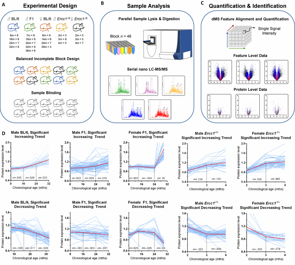
Figure 1.Unbiased detection of age-related changes in protein expression in mouse liver. (A) Details of input tissue samples (age in months and n per group) and methods of bias mitigation for sample preparation and analysis, including the creation of a balanced incomplete block design for all processing and analysis steps and sample blinding. For the Ercc1-/Δ mouse liver the n refers to mutant mice / littermate controls. (B) Sample processing block size and representative mass chromatograms generated from each sample. See methods section for more detail. (C) Alignment, extraction, and storage of mass spectral feature data from raw mass spectrometer output based on retention time and accurate mass, allowing for quantification of each proteomic signal across all samples, results of which are shown in example feature level volcano plots. The y-axis is the negative log of p-value; the x-axis is the log fold-change in protein abundance. All features associated with a protein are combined to calculate protein expression as shown in volcano plots indicating proteins (individual dots) that were significantly increased or decreased in expression in old vs. young mice and the extent of that change in expression. (D) Plots of the relative abundance of all proteins (individual blue lines) that change significantly with aging as identified by one-way ANOVA. Protein expression was measured cross-sectionally throughout the lifespan of inbred male C57BL/6Jnia, male f1a (C57BL6/Jnia:Balb/cBy), female f1b (C57BL/6J:FVB/NJ), male f1b (C57BL/6J:FVB/NJ) Ercc1-/Δ , and female f1b (C57BL/6J:FVB/NJ) Ercc1-/Δ mouse livers. The graphs are separated into proteins that increased in expression with chronological age (top) or decreased (bottom). The red line represents the mean protein abundance for significantly altered proteins in that group. m= the slope between time points. Significance cutoffs as delineated in Supplementary Table 2.