DDX20 and NCBP2 were identified via feature selection algorithms and PPI network analysis
5 genes were identified as important features of NOA through LASSO regression (Figure 4A), including NCBP2, DDX20, TSN, SRPK2, and CARHSP1. The coefficients of these genes in the LASSO regression model were −0.121, −0.703, −0.770, −0.921, and −0.178, respectively (Figure 4B). Simultaneously, 30 of 51 DEGs were selected via the Boruta algorithm (Figure 4C, Supplementary Table 4), and 6 genes, including NCBP2, DDX20, CCDC86, TSN, CARHSP1, and TDRD7, were screened by SVM-RFE (Figure 4D). Ultimately, NCBP2 and DDX20 were identified by integrating the Top 20 genes with the highest degree in the PPI network and these feature selection results (Figure 4E) and then included in the diagnosis model construction.
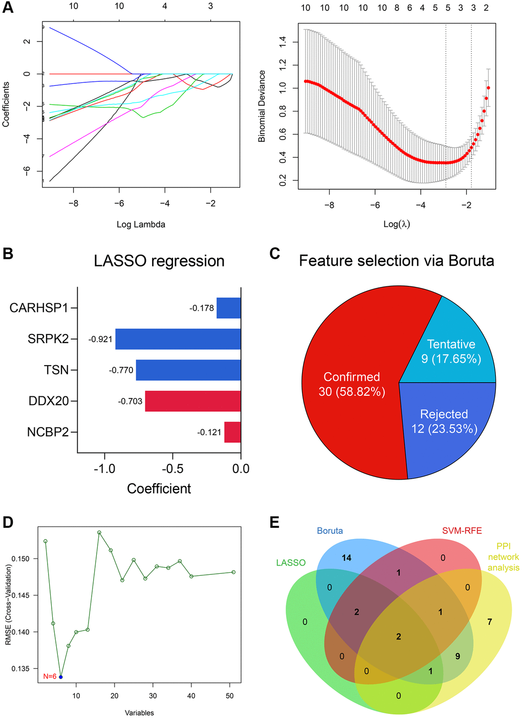
Figure 4. DDX20 and NCBP2 were con-determined via feature selection methods and PPI network analysis. (A) 5 genes, including NCBP2, DDX20, TSN, SRPK2, and CARHSP1, were identified as significant features to NOA via LASSO regression. (B) The coefficients of the 5 selected genes in the LASSO regression model. (C) 30 genes were determined as important features via the Boruta algorithm. (D) 6 genes, including NCBP2, DDX20, CCDC86, TSN, CARHSP1, and TDRD7, were selected by the SVM-RFE. (E) DDX20 and NCBP2 were con-determined by the machine learning algorithms and PPI network analysis.
External validation of DDX20 and NCBP2
The scRNA-seq data of 432 testicular cell samples indicated that DDX20 (Nominal P < 0.001, FDR < 0.001) and NCBP2 (Nominal P < 0.01, FDR < 0.05) were both positively associated with the spermatogenetic process (Figure 5A), re-confirming that DDX20 and NCBP2 were significant biomarkers to NOA. Next, we gleaned the seminal plasma and testicular biopsy of 27 control and 17 NOA patients from the local hospital for validation. Compared with the control samples, the NOA samples exhibited lower mRNA levels of DDX20 (P < 0.01, Figure 5B) and NCBP2 (P < 0.05, Figure 5C) in seminal plasma, suggesting that the levels of DDX20 and NCBP2 in seminal plasma were also promising diagnostic biomarkers for NOA. ROC analysis showed that DDX20 in seminal plasma was a powerful classifier for NOA (area under the curve [AUC] = 0.826, 95% confidence interval [CI] = 0.706–0.946, Figure 5D), while the predictive performance of NCBP2 was relatively low (AUC = 0.693, 95% CI = 0.534–0.852, Figure 5D), which might be caused by the heterogeneity across different cohorts. Hence, we then investigated the protein levels of DDX20 in the local cohort using IHC staining, and the results supported the conclusion drawn before that DDX20 was significantly down-regulated in NOA testicular samples (P < 0.05, Figure 5E).
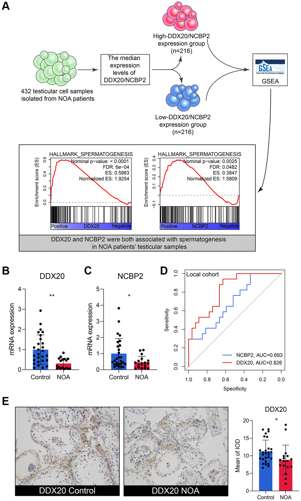
Figure 5. The external validation of DDX20 and NCBP2. (A) The single-cell RNA-sequencing analysis of 432 testicular cell samples isolated from NOA patients displayed that DDX20 and NCBP2 were both positively associated with spermatogenesis. (B, C) DDX20 (B) and NCBP2 (C) were down-regulated in the seminal plasma samples of NOA patients from the local hospital. (D) The ROC curve exhibited the diagnosis ability of seminal plasma DDX20 and NCBP2 to NOA in the local cohort. (E) The protein expression levels of DDX20 were obviously down-regulated in the testicular samples from NOA patients in the local cohort, which were detected by the immunohistochemical staining. Abbreviation: ROC: receiver operating characteristic.
The performance of LR, RF, and ANN diagnosis models
The present study utilized multiple datasets, including GSE9210, GSE45885, GSE45887, and GSE145467, and local clinical samples to verify the predictive ability of the established model. The detailed clinicopathological parameters of the training and external validation cohorts are displayed in Table 3. It should be stated that we used the mRNA expression values in the seminal plasma, other than in the testicular samples, to validate the models in the local cohort because the fresh testicular samples were unavailable given the policy formulated by the ethics committee of our hospital. Since we have detected the expressions of DDX20 and NCBP2 in the seminal plasma and found that both genes were down-regulated in NOA samples, which corresponded to the results in the training dataset, we thought that the validation in the seminal plasma samples from the local cohort was still acceptable.
Table 3. The clinicopathological features of the cohorts enrolled in this study.
| Characteristics | GSE9210 | GSE45885 | GSE45887 | GSE145467 | Local cohort |
| Control (n = 11) | NOA (n = 47) | Control (n = 4) | NOA (n = 27) | Control (n = 4) | NOA (n = 16) | Control (n = 10) | NOA (n = 10) | Control (n = 27) | NOA (n = 17) |
| Age (years) | 33.3 ± 8.5 | 35.0 ± 5.7 | – | 32.1 ± 4.05 | – | 31.3 ± 1.8 | – | – | 31.8 ± 9.2 | 33.4 ± 7.4 |
| Johnsen’s score | 7.9 ± 1.2 | 2.4 ± 1.3 | – | 4.9 ± 2.5 | – | – | – | – | 7.3 ± 1.7 | 2.7 ± 2.5 |
| FSH (mIU/ml) | 10.1 ± 9.3 | 29.2 ± 9.1 | – | – | – | – | – | – | 11.1 ± 7.6 | 21.6 ± 8.8 |
| LH (mIU/ml) | 4.5 ± 2.3 | 8.8 ± 4.8 | – | – | – | – | – | – | 4.3 ± 0.9 | 8.1 ± 3.5 |
| T (ng/ml) | 4.8 ± 1.7 | 3.5 ± 1.6 | – | – | – | – | – | – | 5.1 ± 0.7 | 3.7 ± 1.2 |
| Abbreviations: FSH: follicle-stimulating hormone; LH: luteinizing hormone; T: testosterone; NOA: non-obstructive azoospermia. |
First, an LR diagnosis model was constructed as follows: Score = 10.101–16.148 × EXP(NCBP2) + 0.046 × EXP(DDX20), where the EXP meant the mRNA expression value of the gene. The predictive ability of the LR model in the training cohort was quite high (AUC = 0.955, 95% CI = 0.865–1.000, Figure 6A). However, its performance in the GSE45885 cohort (AUC = 0.514, 95% CI = 0.256–0.772, Figure 6B) and the GSE45887 cohort (AUC = 0.531, 95% CI = 0.267–0.795, Figure 6C) was non-ideal. The AUCs of the LR model in the GSE145467 and local cohorts are 0.700 (95% CI = 0.493–0.907, Figure 6D) and 0.597 (95% CI = 0.465–0.729, Figure 6E), respectively. The confusion matrices of the LR model in these cohorts are shown in Figure 6F–6J, respectively. Generally, the predictive ability of the LR model was far from satisfactory, especially in the external validation cohorts, enlightening us to utilize more tools to construct the diagnosis models.
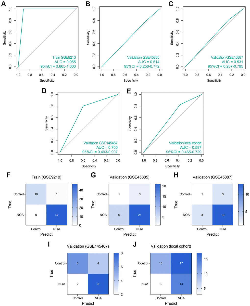
Figure 6. The predictive performance of an LR diagnosis model in each cohort. (A–E) The ROC analyses of the LR model in the training cohort (A), GSE45885 cohort (B), GSE45887 cohort (C), GSE145467 cohort (D), and the local cohort (E). (F–J) The confusion matrices of the LR model in the training cohort (F), GSE45885 cohort (G), GSE45887 cohort (H), GSE145467 cohort (I), and the local cohort (J). Abbreviation: LR: logistic regression.
Subsequently, we established an RF model to classify the NOA samples. The RF model showed superiority to the routine LR model in the training dataset (AUC = 1.000, 95% CI = 1.000–1.000, Figure 7A), GSE45885 dataset (AUC = 0.676, 95% CI = 0.385–0.967, Figure 7B), GSE45887 dataset (AUC = 0.656, 0.381–0.932, Figure 7C), GSE145467 dataset (AUC = 0.750, 95% CI = 0.562–0.938, Figure 7D), and local cohort (AUC = 0.656, 95% CI = 0.547–0.765, Figure 7E). Figure 7F–7J represent the confusion matrices of the RF model in each cohort.
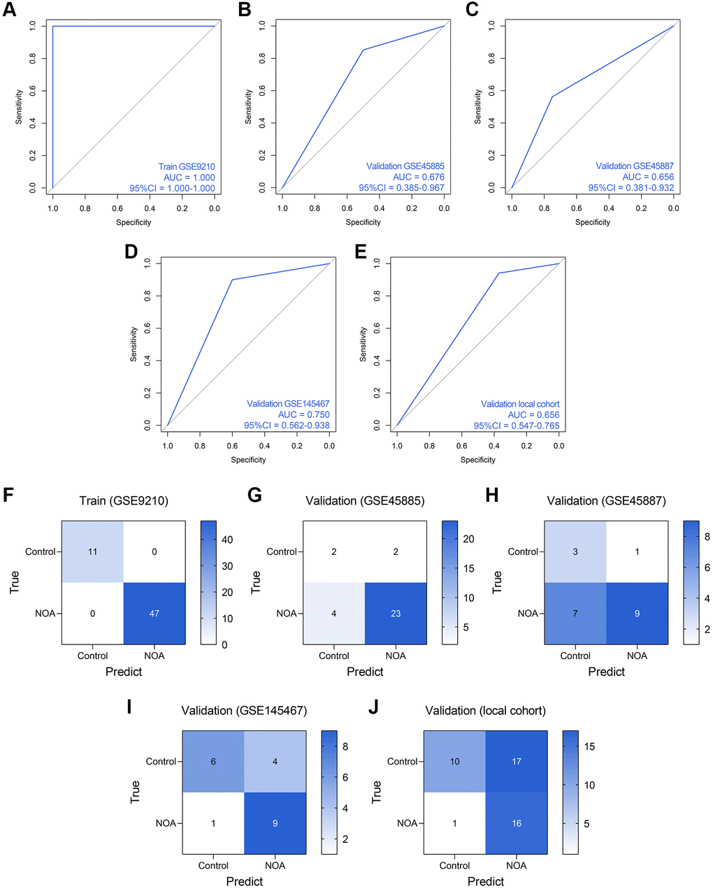
Figure 7. The predictive performance of an RF diagnosis model in each cohort. (A–E) The ROC analyses of the RF model in the training cohort (A), GSE45885 cohort (B), GSE45887 cohort (C), GSE145467 cohort (D), and the local cohort (E). (F–J) The confusion matrices of the RF model in the training cohort (F), GSE45885 cohort (G), GSE45887 cohort (H), GSE145467 cohort (I), and the local cohort (J). Abbreviation: RF: random forest.
ANN was also a widely-used method for diagnosis model establishment, and many ANN diagnosis models have been proposed and exhibited high reliability and precision in multiple diseases [20–22]. Thus, we then developed an ANN diagnosis model based on the expressions of DDX20 and NCBP2 in NOA, as displayed in Figure 8A. Similar to those previous contributions, the established ANN model showed high predictive performance across the training cohort (AUC = 0.840, 95% CI = 0.773–0.908, Figure 8B), GSE45885 cohort (AUC = 0.731, 95% CI = 0.446–1.000, Figure 8C), GSE45887 cohort (AUC = 0.781, 95% CI = 0.517–1.000, Figure 8D), GSE145467 cohort (AUC = 0.850, 95% CI = 0.700–1.000, Figure 8E), and local cohort (AUC = 0.623, 95% CI = 0.482–0.765, Figure 8F). Figure 8G–8K displayed the confusion matrices of these cohorts. The performance of the ANN model in the local cohort was not satisfying (AUC < 0.7), but we held that the result was still acceptable considering the different sample types and gene expression detection methods. As a whole, the ANN model was a promising tool to classify the NOA samples on the background of the high heterogeneity among different cohorts.
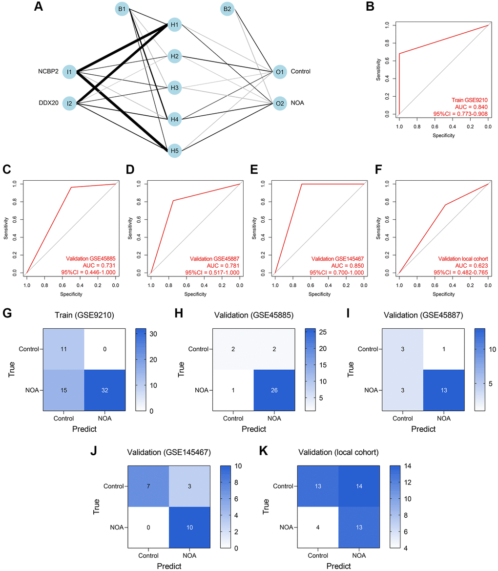
Figure 8. Establishment and validation of an ANN diagnosis model. (A) An ANN model containing one input layer, one hidden layer, and one output layer was constructed to diagnose NOA. (B–F) The ROC analyses of the ANN model in the training cohort (B), GSE45885 cohort (C), GSE45887 cohort (D), GSE145467 cohort (E), and the local cohort (F). (G–K) The confusion matrices of the RF model in the training cohort (G), GSE45885 cohort (H), GSE45887 cohort (I), GSE145467 cohort (J), and the local cohort (K). Abbreviation: ANN: artificial neural network.
Here, we measure the predictive performance of these models mainly from the aspect of AUC. However, the other assessment indexes, containing accuracy, precision, recall, F-measure, sensitivity, specificity, positive predictive value, and negative predictive value, were also provided for reference, as listed in Table 4.
Table 4. The predictive performance of the established models in each cohort.
| Cohort | Accuracy | Precision | Recall | F-measure | Sensitivity | Specificity | Positive predictive value | Negative predictive value |
| Logistic regression model |
| GSE9210 | 0.983 | 0.979 | 1.000 | 0.989 | 1.000 | 0.909 | 0.979 | 1.000 |
| GSE45885 | 0.710 | 0.875 | 0.778 | 0.824 | 0.778 | 0.250 | 0.875 | 0.143 |
| GSE45887 | 0.700 | 0.813 | 0.813 | 0.813 | 0.813 | 0.250 | 0.813 | 0.250 |
| GSE145467 | 0.700 | 0.667 | 0.800 | 0.727 | 0.800 | 0.600 | 0.667 | 0.750 |
| Local Cohort | 0.545 | 0.452 | 0.824 | 0.583 | 0.824 | 0.370 | 0.452 | 0.769 |
| Random forest model |
| GSE9210 | 1.000 | 1.000 | 1.000 | 1.000 | 1.000 | 1.000 | 1.000 | 1.000 |
| GSE45885 | 0.806 | 0.920 | 0.852 | 0.885 | 0.852 | 0.500 | 0.920 | 0.333 |
| GSE45887 | 0.600 | 0.900 | 0.563 | 0.692 | 0.563 | 0.750 | 0.900 | 0.300 |
| GSE145467 | 0.750 | 0.692 | 0.900 | 0.783 | 0.900 | 0.600 | 0.692 | 0.857 |
| Local Cohort | 0.591 | 0.485 | 0.941 | 0.640 | 0.941 | 0.370 | 0.485 | 0.909 |
| Artificial neural network model |
| GSE9210 | 0.741 | 1.000 | 0.681 | 0.810 | 0.681 | 1.000 | 1.000 | 0.423 |
| GSE45885 | 0.903 | 0.929 | 0.963 | 0.945 | 0.963 | 0.500 | 0.929 | 0.667 |
| GSE45887 | 0.800 | 0.929 | 0.813 | 0.867 | 0.813 | 0.750 | 0.929 | 0.500 |
| GSE145467 | 0.850 | 0.769 | 1.000 | 0.870 | 1.000 | 0.700 | 0.769 | 1.000 |
| Local Cohort | 0.591 | 0.481 | 0.765 | 0.591 | 0.765 | 0.481 | 0.481 | 0.765 |