Results related to tumor stem cell scoring
The content of tumor stem cells in tumor tissues had a strong correlation with tumor recurrence, often leading to poor prognosis. The prediction results of tumor stem cell content (mRNAsi) of TCGA samples by Malta et al were used to evaluate the content of tumor stem cells in samples [16]. The mRNAsi was analyzed in different clinical traits. A significant difference (Wilcoxon test, P < 0.001) in mRNAsi was found between LIHC samples and normal samples (Figure 2A). mRNAsi did not differ significantly in different ages, genders, and tumor stages (Supplementary Figure 2A–2C). In different tumor grades, mRNAsi has significant differences (Figure 2B, Wilcoxon test, P=0.006), and with the increase of grade, the mRNAsi score gradually increases, which shows that mRNAsi can fully reflect the tumor cell differentiation status. The data of patients with LIHC obtained from TCGA were grouped according to the median mRNAsi value, and the Kaplan–Meier test was performed for survival analysis to explore the relationship between mRNAsi and patient prognosis. Patients with low mRNAsi scores had a better prognosis (Figure 2C, P=0.006). The results showed that it was reasonable to use mRNAsi to evaluate the tumor stem cell content in LIHC samples and normal samples.
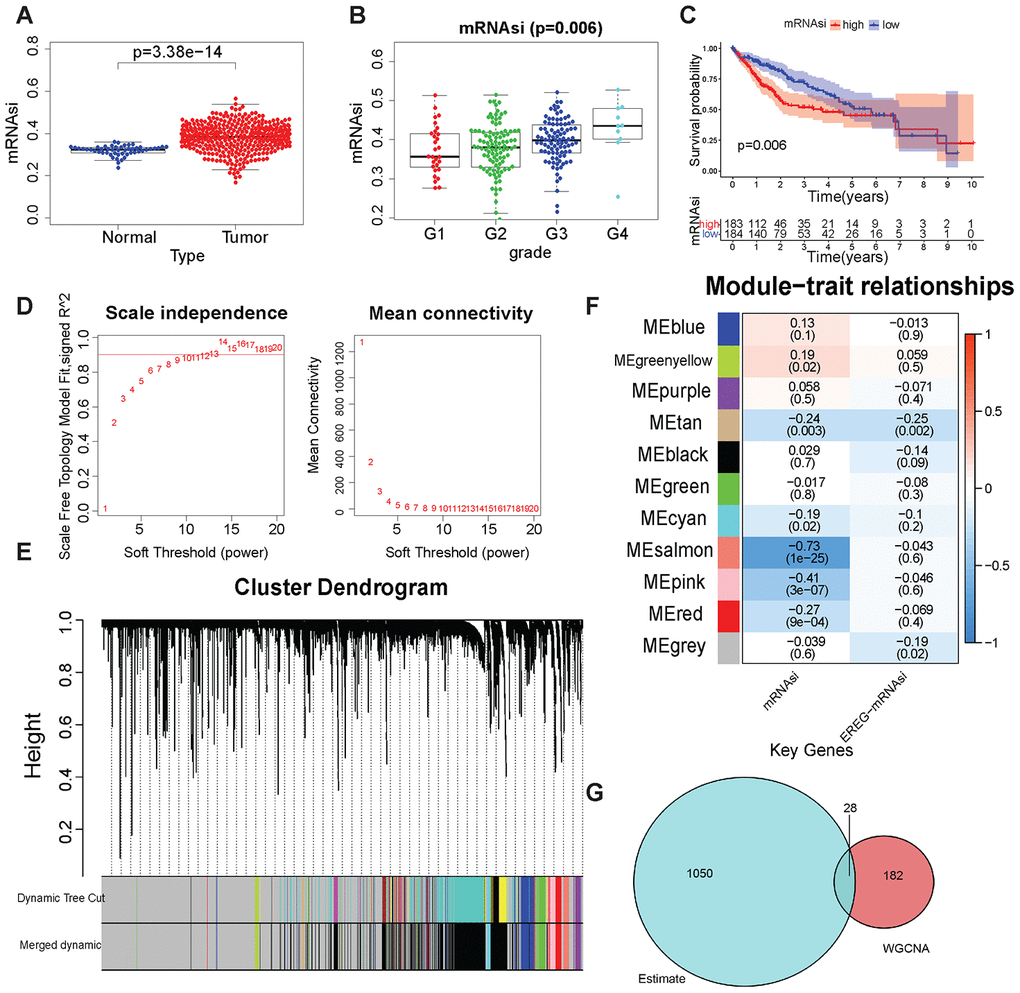
Figure 2. Tumor stem cell score and WGCNA-related results. (A) mRNAsi in LIHC and normal samples. (B) mRNAsi was in different grades. (C) Kaplan–Meier plot of high- or low-mRNAsi patients from TCGA. The number of patients remaining at a particular time point is shown at the bottom. (D) Left: The determination coefficient R2 of the y-axis is −log10 (k) and log10 (P(k)). The larger the R2, the more the gene regulatory network conformed to the scale-free network. k, Connectivity of the gene nodes; P(k), probability of such a node. Red line: 0.9. The x-axis is the soft threshold beta. Right: the average connectivity of the y-axis genes. The x-axis is the soft threshold β. (E) Gene clustering and gene module partition results. Gene clustering and gene module division results. “Dynamic Tree Cut” is the result before the modules were merged; “Merged dynamic” is the result after the modules were merged. (F) The result of the module–trait relationship. The Pearson correlation coefficient of the first principal component of the gene module and the traits was plotted as a heat map, where the P values are marked in parentheses. (G) The intersection of the ESTIMATE algorithm and mRNAsi + WGCNA-derived genes. These 28 genes were considered to be closely related to the tumor stem cell content and the degree of immunity.
DEGs in 50 normal tissues and 374 LIHC tissues were first screened to find genes in LIHC samples that were closely related to disease occurrence and tumor stem cell scoring. A total of 7273 upregulated genes and 394 downregulated genes were obtained in tumor tissues (Supplementary Figure 2D and 2E). Then, these DEGs were used for WGCNA and mRNAsi as the phenotype for analysis. In this study, when the soft threshold β = 13, the gene regulatory network better met the scale-free network (Figure 2D). First, 7667 DEGs were used to perform hierarchical clustering on 374 LIHC samples. Samples with “Height” greater than 1500 were regarded as outliers and excluded (Supplementary Figure 3A, 3B). Then, the genes were clustered and the gene modules were merged. The “mergeCutHeight” value was set to 0.4 to merge the different gene modules obtained (Supplementary Figure 4A). Figure 2E shows the results of gene clustering. “Dynamic Tree Cut” shows the gene modules before merging, and “Merged dynamic” shows the gene modules after merging. The correlation between the mRNAsi and the first principal component of the gene modules (Pearson's correlation coefficient) is shown in Figure 2F. The pink module (–0.41, P < 0.001) and the salmon module (–0.73, P < 0.001) were closely related to mRNAsi. Moreover, both correlation coefficients were negative, indicating that a high expression of genes in these modules meant lower mRNAsi scores. The relationship between gene expression, phenotype, and the first principal component of the pink and salmon modules are shown in Supplementary Figure 4B and 4C.
Establishment of the prognostic model
The coefficients of the pink and salmon modules obtained by WGCNA were negative (Figure 2F), indicating that the high expression of genes in these two modules represented a decrease in tumor stem cells. The high expression of upregulated genes obtained by the ESTIMATE algorithm meant an increase in the content of immune cells. The reduction in stem cells and the increase in immune cell content were often closely related. Therefore, for finding genes closely related to tumor stem cell content and tumor immune processes, 210 genes in the salmon and pink modules were intersected with 1078 upregulated genes in the ESTIMATE algorithm and 28 key genes were obtained. These 28 genes were used in the construction of subsequent prognostic models. Besides these 28 genes, 14 types of clinical information were also included in the prognostic model to make the prognostic model more informative. A total of 225 patients were then grouped into a training set (n = 114) and a test set (n = 111). The clinical baseline data and grouping of patients are shown in Table 1. The differences in clinical variables between the training set and the test set were examined to illustrate the rationality of random grouping. The chi-square test was used for discrete variables, while the Wilcoxon test was used for continuous variables. Albumin showed a significant difference between the training and test sets (Table 1, P < 0.05), while the other variables showed no significant difference. It was reasonable to have few different variables when grouping because a variety of clinical information was included.
Table 1. Clinical baseline data for patients with LIHC.
| Characteristic | Train sets (n=114) | Test sets (n=111) | t/χ2 value | P value |
| Age | 59.07±12.45 | 59.28±12.33 | -0.1266 | 0.8994 |
| Gender (%) | | | 0.0784 | 0.3098 |
| Female | 40 (35.1) | 36 (32.4) | | |
| Male | 74 (64.9) | 75 (67.6) | | |
| Grade (%) | | | 3.2991 | 0.3098 |
| G1 | 14 (12.3) | 7 (6.3) | | |
| G2 | 47 (41.2) | 55 (49.5) | | |
| G3 | 46 (40.4) | 44 (39.6) | | |
| G4 | 7 (6.1) | 5 (4.5) | | |
| Stage (%) | | | 6.8583 | 0.3098 |
| I | 74 (64.9) | 56 (50.5) | | |
| II | 27 (23.7) | 29 (26.1) | | |
| III+IV | 13 (11.4) | 26 (23.4) | | |
| Race (%) | | | 2.3435 | 0.3098 |
| ASIAN | 59 (51.8) | 55 (49.5) | | |
| BLACK | 6 (5.3) | 2 (1.8) | | |
| WHITE | 49 (43.0) | 54 (48.6) | | |
| Height | 165.85±9.06 | 166.29±13.06 | -0.2925 | 0.7702 |
| Weight | 70.82±17.39 | 74.93±22.36 | -1.5425 | 0.1244 |
| BMI | 25.64±5.47 | 27.6±12.06 | -1.5778 | 0.116 |
| Album | 3.67±1.01 | 3.98±1.05 | -2.2608 | 0.0247 |
| Bilirubin | 0.75±0.41 | 0.92±0.97 | -1.6711 | 0.0961 |
| Creatinine | 1.0±0.67 | 1.6±5.1 | -1.2366 | 0.2176 |
| Fetoprotein | 8590.99±37146.93 | 22260.09±193511.36 | -0.7404 | 0.459 |
For 28 + 14 variables, lasso regression was first performed to eliminate collinearity between the variables. When the penalty coefficient λ = 0.064, the equation had the smallest error (Supplementary Figure 6A), and the coefficients of nine variables were not 0 (Supplementary Figure 6B). Nine variables were used to build a multivariate Cox regression model, and the independent variable selection method was the back-off method. Finally, eight variables were included in the Cox regression model (Figure 4A). model contains clinical information and genes related to the immune process and CSC, we call this model Immunity and CSC related prognosis (ICRP) score. The formula of the ICRP score was as follows:
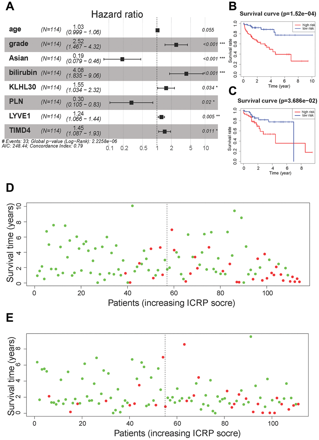
Figure 4. Cox regression model results. (A) A forest plot of the multivariate Cox regression model. Hazard ratio is provided in the figure. (B) The survival curve of the ICRP score in the training set. Grouping was based on the median ICRP score in the training set. Red is the high-level group, and blue is the low-level group. (C) The survival curve of the ICRP score in the test set. Grouping was based on the median ICRP score in the training set. (D) Patient survival status in the training set. The x-axis is the patient ranking in ascending order by the ICRP score; the y-axis is the survival time. The red dots are the dead patients, and the green dots are the surviving patients. (E) Patient survival status in the test set.

Where Age is in year; Grade is an integer from 1 to 4; Asian takes values 1 (means “yes”) and 0 (means “no”); and Bilirubin is in mg/dL; the levels of the four genes are the normalized values of FPKM.
The training and test sets were grouped according to the median value (1.08) of the ICRP score in the training set. All patients with an ICRP score less than 1.08 were in the low-risk group, while all patients with an ICRP score greater than 1.08 were in the high-risk group. Moreover, Kaplan–Meier curves were plotted for survival analysis. The high ICRP score had less survival time in both the training set (Figure 4B, P < 0.001) and the test set (Figure 4C, P < 0.05). In the training set, the 1- and 3-year OS rate was 94.2% (95% CI = 88.0–100.0) and 85.5% (95% CI = 70.7–98.1) in the low-risk group and 76.6% (95% CI = 66.2–88.6) and 56.9% (95% CI = 44.0–73.6) in the high-risk group, respectively. In the test set, the 1- and 3-year OS rates were 92.2% (95% CI = 85.1–99.8) and 81.8% (95% CI = 70.8–94.6) in the low-risk group and 84.8% (95% CI = 75.6–95.1) and 48.9% (95% CI = 31.3–66.5) in the high-risk group, respectively.
The patients were sorted according to the ICRP score, and the distribution of patient survival status was plotted. In the training set (Figure 4D) and test set (Figure 4E), the survival time of patients gradually decreased and the number of death cases gradually increased with the increase in the ICRP score.
Verification of the ICRP score
In order to further verify the effectiveness of our prognostic model and compare it with other method, we used ICRP score, AJCC stage and ALBI score in the training set and test set to predict the survival status of patients at 1, 3, and 5 years, respectively, and plotted the receiver operator characteristic curves. The area under the curve (AUC) of ICRP score in the test set for 1, 3, and 5 years was 0.708, 0.723, and 0.765 respectively (Figure 5A–5C); the AUC of AJCC stage in the test set for 1, 3, and 5 years was 0.584, 0.660, and 0.701, respectively (Figure 5D–5F); the AUC of ALBI score in the test set for 1, 3, and 5 years was 0.654, 0.615, and 0.583, respectively (Figure 5G–5I). The AUCs of ICRP score in the training set for 1, 3, and 5 years was 0.840, 0.801, and 0.824 respectively (Supplementary Figure 6C–6E); the AUCs of AJCC stage in the training set for 1, 3, and 5 years was 0.592, 0.599, and 0.582 (Supplementary Figure 6F–6H); the AUCs of ALBI score in the training set for 1, 3, and 5 years was 0.641, 0.549, and 0.529 (Supplementary Figure 6I–6K). It can be seen that ICRP score’s prediction ability was better than AJCC stage and ALBI score. To further demonstrate this, the C-index of the ICRP score, AJCC stage, and ALBI score in the training and test sets were calculated. The related results are shown in Table 2. It was obvious that the C-index of the ICRP score was significantly larger than the C-index of the AJCC stage and ALBI score in the training set (P < 0.05) and the test set (P < 0.05). Carter et al [27] used the TCGA data to establish a signature that could measure chromosomal instability in tumor cells based on the expression of 25 genes, namely CIN25. They proved that CIN25 was an effective prognostic indicator for many cancers [29, 30]. The CIN25 score of each sample was calculated and the patient's prognosis was predicted. The C-index of CIN25 was significantly lower than that of the ICRP score in the training set (P < 0.05, Table 2) and test set (P < 0.05, Table 2). The aforementioned results showed that the proposed prognostic model was effective.
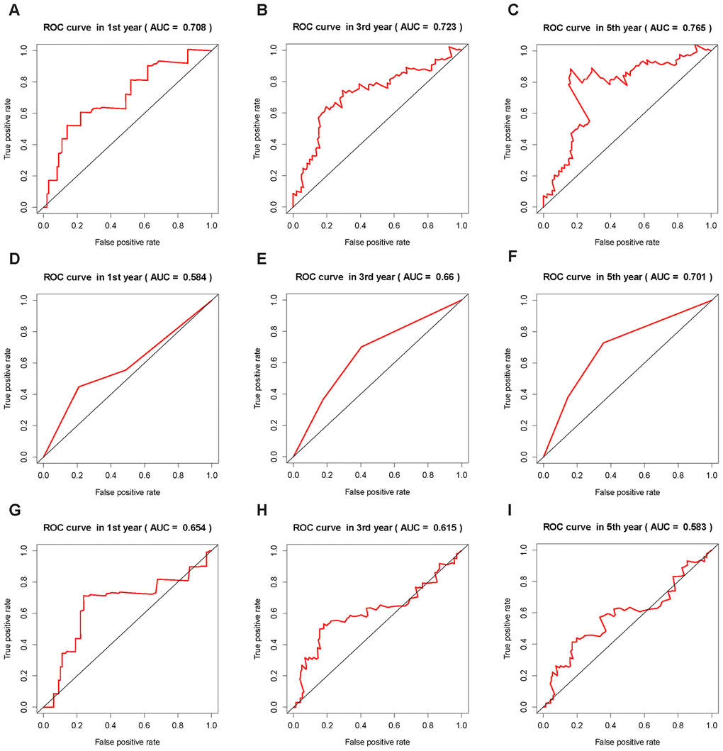
Figure 5. ROC curves of the ICRP score, AJCC stage, and ALBI score. The AUC value is in brackets. (A–C) ROC curves of ICRP score’s forecast result after 1, 3, and 5 years in the test set. (D–F) ROC curves of AJCC stage forecast result after 1, 3, and 5 years in the test set. (G–I) ROC curves of ALBI score prediction results after 1, 3, and 5 years in the test set.
Table 2. C-index results of the ICRP score, AJCC stage, ALBI score, and CIN25.
| Method | Training set | | Test set | |
| C-index(95%CI) | P | C-index(95%CI) | P |
| ICRP score | 0.793(0.713,0.872) | | 0.697(0.587,0.807) | |
| AJCC stage | 0.561(0.467,0.655) | <0.05 | 0.570(0.455,0.687) | <0.05 |
| ALBI score | 0.602(0.510,0.694) | <0.05 | 0.605(0.536,0.674) | <0.05 |
| CIN25 | 0.643(0.579,0.707) | <0.05 | 0.627(0.564,0.690) | <0.05 |
In addition, the genes selected in the ICRP score might have false-positive results. Therefore, a sensitivity test was conducted on the genes in the ICRP score. We used 28 randomly selected genes from DEGs in LIHC patients and 14 kinds of clinical information to construct a new prognostic model applying the same process and parameters, and repeated three times. The C-indexes of the three reconstructed prognostic models were calculated and compared with that of the ICRP score. The results of the ICRP score for the training and test sets were significantly greater than those of the three models (P < 0.05, Table 3), indicating that the genes selected using the mRNAsi score, WGCNA, and ESTIMATE methods were credible.
Table 3. Sensitivity test results of genes in the ICRP score.
| model ID | term | coef | HR | HR.95L | HR.95H | pvalue | C index in training set | P | C index in test set | P | Randomly selected genes |
| model 1 | Asian | -1.790 | 0.167 | 0.063 | 0.443 | 0.000 | 0.699±0.054 | <0.05 | 0.556±0.050 | <0.05 | P2RY10 TRBV4-1 PLXNA4 HOXB3 C1QA PCDH7 PLA2G4A PLCB2 CNTN4 RHBG KLK4 PTPRB COL12A1 HAPLN3 GLUL TRDV1 AC011479.1 FAM83E KRT19 COL4A2 ANOS1 BX649601.1 IGHJ3 CSPG4 PTGIR ELK3 MYCT1 ADAMTS12 |
| fetoprotein | -0.557 | 0.573 | 0.300 | 3.000 | 0.095 | | | | |
| CNTN4 | -2.772 | 0.063 | 0.002 | 2.121 | 0.093 | | | | |
| model 2 | grade | 1.215 | 3.370 | 1.819 | 6.245 | 0.000 | 0.712±0.038 | <0.05 | 0.569±0.053 | <0.05 | TGFA CD300A MFGE8 SLFN12L PDZRN3 FEZ1 GLUL TRIM22 ID3 SELL MMRN2 GPRIN3 NCF1B CXCL14 KCNN3 PSCA C1QTNF3 TRBV4-1 VIM RAB25 POU2F2 DNAJB3 FCRLA IGHV1-69 ADCY3 HOXB3 ARHGAP25 NCF2 |
| stage | 0.576 | 1.780 | 1.115 | 2.841 | 0.016 | | | | |
| Asian | -2.272 | 0.103 | 0.037 | 0.289 | 0.000 | | | | |
| height | -0.058 | 0.944 | 0.909 | 0.980 | 0.003 | | | | |
| TRBV4-1 | 0.612 | 1.844 | 1.112 | 3.058 | 0.018 | | | | |
| HOXB3 | -0.667 | 0.513 | 0.211 | 1.248 | 0.084 | | | | |
| GLUL | -0.001 | 0.999 | 0.998 | 1.000 | 0.083 | | | | |
| model 3 | age | 0.057 | 1.058 | 1.018 | 1.100 | 0.004 | 0.678±0.066 | <0.05 | 0.597±0.060 | <0.05 | C1QTNF7 CST7 CDX1 TRAV12-3 AC090409.1 TRBV7-6 TGFB2 HLA-DQA2 BHLHE22 AC119044.1 DGKA AEBP1 PEG10 PTGIS ST8SIA4 GALNT5 ICAM3 SRGN HBD CSF1R RAB31 LRRC4 ZNF469 TUBB6 ZBP1 MYOM2 STEAP4 AC002398.2 |
| grade | 1.330 | 3.780 | 1.759 | 8.124 | 0.001 | | | | |
| Asian | -1.028 | 0.358 | 0.113 | 1.133 | 0.080 | | | | |
| BMI | 0.045 | 1.046 | 1.005 | 1.088 | 0.026 | | | | |
| CDX1 | -1.237 | 0.290 | 0.085 | 0.657 | 0.094 | | | | |
| CSF1R | 0.037 | 1.038 | 0.998 | 1.080 | 0.063 | | | | |
Next, qPCR experiments were used to check the change in gene expression level in normal cell line (THLE3) and LIHC cell line (SNU-423). As shown in Figure 6A, gene expression of KLHL30 and PLN significantly changed, while no significant difference was observed in the expression levels of LYVE1 and TIMD4 (Supplementary Figure 7). To some extent, the results of qPCR proved the difference in the expression of these genes in different cell lines. Moreover, the Human Protein Atlas database was used to further understand the functions of these significant genes in the ICRP score model. The related IHC results showed that the expression of PLN was upregulated in tumor tissues while the expression of LYVE1 and TIMD4 were down-regulated (Figure 6B–6D, KLHL30 was not found in this database), which indicated these genes do have expression variation in protein level during the development of liver cancer. Detailed information on IHC results was shown in Supplementary Table 2. Furthermore, the study explored whether the aforementioned significant factors had a strong correlation with the ICRP score. Hence, the chi-square test for discrete variables and U test for continuous variables were performed in both training and test sets. Age, Asian, bilirubin, and PLN had a strong difference between high–ICRP score and low–ICRP score groups, while grade was significant in the test set than in the training set (Figure 6E–6H). To observe the relationship of these four genes and immune infiltration, TIMER database (https://cistrome.shinyapps.io/timer/) was used to calculate the correlation between the genes and different immune cells to observe the relationship of these four genes with immune infiltration. As shown in Figure 7, KLHL30 expression was positively associated with the infiltration of B cells (Cor = 0.122, P = 0.023), CD8+ T cells (Cor = 0.228, P = 2e-05), CD4+ T cells (Cor = 0.398, P = 1.75e-14), macrophages (Cor = 0.421, P = 4.34e-16), neutrophils (Cor = 0.384, P = 1.52e-13), and dendritic cells (Cor = 0.271, P = 3.94e-07). The PLN expression was closely associated with the infiltration level of CD8+ T cells (Cor = 0.171, P = 0.001), CD4+ T cells (Cor = 0.326, P = 6.01e-10), macrophages (Cor = 0.236, P = 1.03e-05), neutrophils (Cor = 0.208, P = 0.0001), and dendritic cells (Cor = 0.247, P = 4.21e-06). The LYVE1 expression was positively related to the infiltration of CD8+ T cells (Cor = 0.176, P = 0.001), CD4+ T cells (Cor = 0.133, P = 0.013), macrophages (Cor = 0.303, P = 1.14e-08), neutrophils (Cor = 0.272, P = 3.03e-07), and dendritic cells (Cor = 0.164, P = 0.002). A positive correlation was found between the TIMD4 expression level and the infiltration of B cells (Cor = 0.312, P = 3.43e-09), CD8+ T cells (Cor = 0.361, P = 6.03e-12), CD4+ T cells (Cor = 0.198, P = 2.26e-4), macrophages (Cor = 0.303, P = 1.14e-08), neutrophils (Cor = 0.293, P = 3.02e-08), and dendritic cells (Cor = 0.397, P = 2.75e-14). The results indicated that the aforementioned four genes related to prognosis had a strong correlation with immune process, explaining why these genes could be used as biomarkers in LIHC prognosis. Previous studies [31] showed that the number of activated monocytes and plasma cells decreased and the numbers of B cells, CD4+ T cells, and CD8+ T cells increased in LIHC, compared with the healthy liver. This was consistent with the results of the present study. It is generally believed that B cells can be used as antigen-presenting cells to induce CD4+ T cell–dependent CD8+ memory T cells [32], thereby helping to control tumor invasion and metastasis.
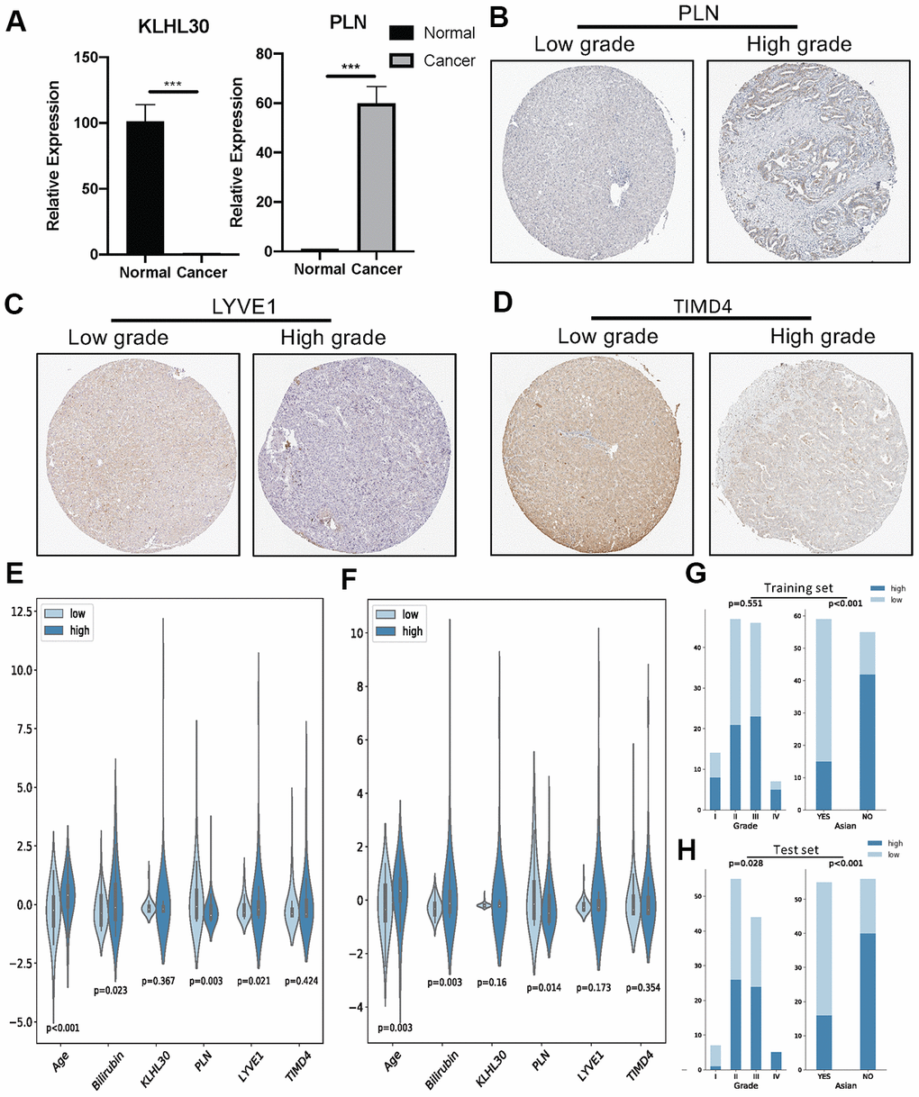
Figure 6. (A) QPCR analysis of KLHL30 and PLN in normal liver cell line and LIHC cell line (n = 3, ***P < 0.001, paired t test. (B–D) IHC results related to significant genes. (E) Nonparametric test (U test) for continuous variables and risk groups in the training set; P < 0.05 represents significant difference. (F) U test for continuous variables and risk groups in the test set; P < 0.05 represents significant difference. (G and H) Chi-square test for discrete variables and risk groups. (G) Training set. (H) Test sets. P < 0.05 represents a significant difference.
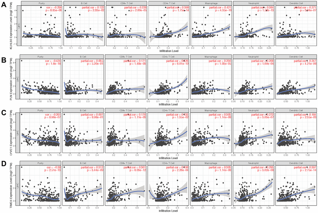
Figure 7. Scatter plot of gene expression and immune cell content. (A–D) show the relationship between the expression levels of KLHL30, PLN, LYVE1, and TIMD4 and the content of immune cells, respectively.