


Introduction
Prostate cancer is the second most commonly diagnosed cancer and the sixth leading cause of cancer-related death in men [1]. Early diagnosis and treatment are of great importance. Serum prostate-specific antigen (PSA) detection is the primary option for screening prostate cancer [2]. However, PSA is specific to prostate tissue rather than tumor tissue, and prostatitis, urinary tract infection and even prostate massage can lead to an increase in PSA levels. It has been reported that the specificity of PSA is very low when 4.0 ng/ml serum PSA is used as a threshold [3]. PSA detection alone may cause a high false-positive rate and lead to a large number of unnecessary biopsies [4]. Therefore, PSA-based screening for prostate cancer is controversial.
In clinical practice, magnetic resonance imaging (MRI) has been widely used to detect prostate cancer. It differs from other techniques such as computed tomography and ultrasound since it produces excellent soft tissue contrast without harmful ionizing radiation; MRI also provides imaging evidence for the clinical examination of prostate cancer location, staging, postoperative follow-up, and the evaluation of tumor invasion [5]. MRI mainly included five imaging parameters: T1-weighted imaging, T2-weighted imaging, diffusion-weighted imaging (DWI), magnetic resonance spectroscopy, and dynamic contrast-enhanced imaging. DWI can estimate morphological changes in prostate tissue that occur with the induction of plasticity by probing water diffusion and can qualitatively and quantitatively evaluate the cellular and histological structure of prostate cancer [6]. The b-value is one of the primary parameters influencing DWI results. According to the Prostate Imaging Reporting and Data System version 2, high b-values (1,400–2,000 s/mm2) are favored over standard b-values (800–1,000 s/mm2) for improving tumor detection since they can qualitatively distinguish lesions and normal prostate tissue. The latter shows high signal intensity on DWI, which may not be suppressed even at a b-value of 1,000 s/mm2, resulting in obscured prostate cancer [7, 8]. Higher b-value DWI has been continuously applied in clinical practice. Although a high b-value reduces the signal-to-noise ratio of images and may distort images, it can reduce the T2 penetration effect and microcirculation perfusion of images and more truly reflect the tissue and cytological structure. Because of conflicting results from qualitative and quantitative studies, it is not definitively known whether high b-value DWI improves the diagnostic accuracy of prostate cancer. The purpose of this meta-analysis was therefore to assess the diagnostic performance of high b-value DWI for detecting prostate cancer.
Results
Search process and general characteristics
A flow chart of the study selection process is shown in Figure 1. A total of 641 articles were retrieved during the original search of publications from January 1, 1995, to December 31, 2020, and 233 remained after excluding duplicates among the different databases during the second search round. After excluding reviews, comments, case reports, and studies unrelated to our topics, 61 articles were reviewed. Twenty-four articles remained after omitting articles that did not mention diagnostic accuracy or that had insufficient data [9–32], [13–36]. The excluded studies with reasons are provided in Supplementary Material 1. The backgrounds and designs of these studies are shown in Table 1 and Table 2. Thirteen studies selected populations with PCa, and two studies were performed on suspected cases. The methods for identifying b-values were different: ten studies used motion-probing gradients, and five studies used signal extrapolation by fitting models. All DWI scans were acquired using single-shot spin-echo echo-planar imaging. The biopsy types included targeted biopsy, prostatectomy and systematic biopsy. The used tissue amounts were hardly reported in the studies. The primary characteristics of the selected studies are shown in Table 3. Among the enrolled studies, 17 were prospective studies and 7 were retrospective studies. Among the studies, a total of 1887 patients with 11374 lesions were analyzed. The mean age of all patients was 66.3 years. The MRI field intensity used in most of the studies was 3.0 T, with only three studies using a field intensity of 1.5 T. An endorectal coil was used in only two study. Table 1 also lists the MRI suppliers, gold standards, and DWI diagnostic measures. Table 2 shows that each study contained a b-value of 2,000 s/mm2, and the highest b-value was 4,500 s/mm2. The ranges of the sensitivities and specificities in all studies were 44.0–98.6% and 50.0–99.4%, respectively.
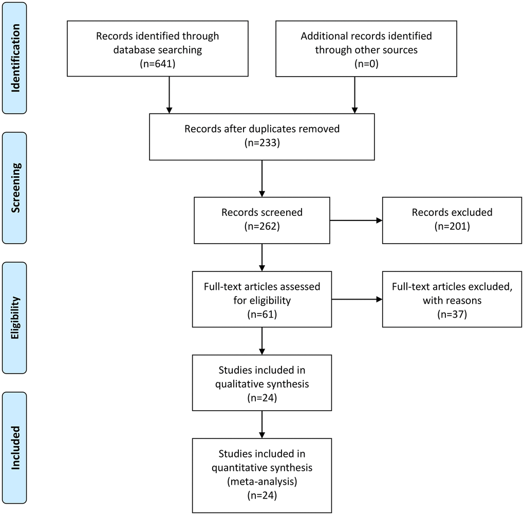
Figure 1. Flow diagram of studies selection process.
Table 1. Background and design information of included studies in the meta–analysis.
| Author | Country | Study design | Patients | Mean age (y) | b-value | PSA(μg/L) | Field Intensity(T) | MRI Supplier | Endorectal Coil | DWI diagnostic measure | |||||||||||||||||||||||||||||||||||||||||||||||||||||||||||||||||||||||||||||||||||||||||
| Adubeio | Portugal | prospective | 43 | 63 | 0,50,100,150,200,500,800,1100,1400, 1700,2000 | – | 3.0 | Philips | No | Visual evaluation | |||||||||||||||||||||||||||||||||||||||||||||||||||||||||||||||||||||||||||||||||||||||||
| Barral | France | prospective | 35 | 64 | 0.2000 | – | 3.0 | Siemens | No | Visual evaluation | |||||||||||||||||||||||||||||||||||||||||||||||||||||||||||||||||||||||||||||||||||||||||
| Wang | China | prospective | 67 | 68.3 | 0,800,1500,2000 | 6.50~530 | 3.0 | Philips | No | Visual evaluation | |||||||||||||||||||||||||||||||||||||||||||||||||||||||||||||||||||||||||||||||||||||||||
| Li | China | prospective | 47 | 68 | 0,400,1000,1500,2000 | – | 3.0 | Siemens | No | Visual evaluation | |||||||||||||||||||||||||||||||||||||||||||||||||||||||||||||||||||||||||||||||||||||||||
| Koo | Korea | retrospective | 80 | 66 | 0,300,700,1000,2000 | 1.24~56.98 | 3.0 | Philips | No | Visual evaluation | |||||||||||||||||||||||||||||||||||||||||||||||||||||||||||||||||||||||||||||||||||||||||
| Feng | China | prospective | 56 | 66.71 | 0,1000,2000,3200, 4500 | 2.06~1000 | 3.0 | GE | No | ADC value | |||||||||||||||||||||||||||||||||||||||||||||||||||||||||||||||||||||||||||||||||||||||||
| Kim | Korea | retrospective | 48 | 66 | 0,1000,2000 | 2.30~23.2 | 3.0 | Philips | No | Visual evaluation | |||||||||||||||||||||||||||||||||||||||||||||||||||||||||||||||||||||||||||||||||||||||||
| Wang | China | prospective | 80 | 66 | 0,300,700,1000,2000 | 1.24~56.98 | 3.0 | GE | No | Visual evaluation | |||||||||||||||||||||||||||||||||||||||||||||||||||||||||||||||||||||||||||||||||||||||||
| Zhang | China | prospective | 40 | 67 | 0,1000,2000,3000 | – | 3.0 | GE | No | Visual evaluation | |||||||||||||||||||||||||||||||||||||||||||||||||||||||||||||||||||||||||||||||||||||||||
| Peng | USA | retrospective | 48 | 62.5 | 0,50,200,1000,1500, 2000 | 0.80~256 | 1.5 | Philips | Yes | ADC | |||||||||||||||||||||||||||||||||||||||||||||||||||||||||||||||||||||||||||||||||||||||||
| Meng | China | prospective | 80 | 72.45 | 0,1000,2000 | – | 3.0 | GE | No | ADC | |||||||||||||||||||||||||||||||||||||||||||||||||||||||||||||||||||||||||||||||||||||||||
| Zhang | China | retrospective | 170 | 59.5 | 0,600,800,1000,1500. 2000,2500,3000 | – | 1.5 | GE | No | Visual evaluation | |||||||||||||||||||||||||||||||||||||||||||||||||||||||||||||||||||||||||||||||||||||||||
| Ning | China | retrospective | 97 | 64 | 0,1200,2000 | 0.60~63 | 3.0 | GE | No | Visual evaluation | |||||||||||||||||||||||||||||||||||||||||||||||||||||||||||||||||||||||||||||||||||||||||
| Wang | China | prospective | 60 | 85.5 | 0,2000 | 4.10~150.2 | 3.0 | Siemens | No | Visual evaluation | |||||||||||||||||||||||||||||||||||||||||||||||||||||||||||||||||||||||||||||||||||||||||
| Xue | China | prospective | 37 | 62 | 0,500,1000,1500,2000 | 3.06~153 | 3.0 | Philips | No | ADC | |||||||||||||||||||||||||||||||||||||||||||||||||||||||||||||||||||||||||||||||||||||||||
| Costa | USA | Prospective | 49 | 61 | 0.2000 | 0.9–26 | 3.0 | - | both | Visual evaluation | |||||||||||||||||||||||||||||||||||||||||||||||||||||||||||||||||||||||||||||||||||||||||
| Katahira et al. | Japan | retrospective | 201 | 69 | 0,1000.2000 | 2.6–114 | 1.5 | Philips | No | Visual evaluation | |||||||||||||||||||||||||||||||||||||||||||||||||||||||||||||||||||||||||||||||||||||||||
| Ohgiya | Japan | retrospective | 73 | 70 | 0,500.1000,2000 | 11.7 | 3 | Siemens | No | Visual evaluation | |||||||||||||||||||||||||||||||||||||||||||||||||||||||||||||||||||||||||||||||||||||||||
| Rosenkrantz | USA | retrospective | 106 | 62 | 50,1000,2000 | 4.5–130 | 3 | Siemens | No | Visual evaluation | |||||||||||||||||||||||||||||||||||||||||||||||||||||||||||||||||||||||||||||||||||||||||
| Stanzione | Italy | Prospective | 82 | 65 | 0,400,2000 | 8.8 | 3 | Siemens | No | Visual evaluation | |||||||||||||||||||||||||||||||||||||||||||||||||||||||||||||||||||||||||||||||||||||||||
| Thestrup | Denmark | retrospective | 204 | 64.1 | 0,1000,2000 | 2.2–120 | 3 | Philips | No | Visual evaluation | |||||||||||||||||||||||||||||||||||||||||||||||||||||||||||||||||||||||||||||||||||||||||
| Ueno1 | Japan | retrospective | 73 | 67 | 0,1000,2000 | 2.9–49 | 3 | Philips | No | Visual evaluation | |||||||||||||||||||||||||||||||||||||||||||||||||||||||||||||||||||||||||||||||||||||||||
| Ueno2 | Japan | retrospective | 80 | 67 | 0,1000,2000 | 2.9–49 | 3 | Philips | No | Visual evaluation | |||||||||||||||||||||||||||||||||||||||||||||||||||||||||||||||||||||||||||||||||||||||||
| Ueno | Japan | retrospective | 31 | 65 | 0,2000 | 4.7–16.5 | 3 | Philips | No | Visual evaluation | |||||||||||||||||||||||||||||||||||||||||||||||||||||||||||||||||||||||||||||||||||||||||
| Abbreviations: PSA: prostate-specific antigen; MRI: magnetic resonance imaging; DWI: diffusion-weighted imaging; TRUS: transrectal ultrasound; TSB: tissue sample biopsy; RP: radical prostatectomy; ADC: apparent dispersion coefficient. | |||||||||||||||||||||||||||||||||||||||||||||||||||||||||||||||||||||||||||||||||||||||||||||||||||
Table 2. Technology characteristics of included study.
| Author | Population | Biopsy type | Type of sequences | TR/TE (ms) | Diffusion times | Methods for identifying | |||||||||||||||||||||||||||||||||||||||||||||||||||||||||||||||||||||||||||||||||||||||||||||
| Adubeio | PCa | Targeted/prostatectomy | SS-SE-EPI | 3258/66 | 13:21 min | signal extrapolation | |||||||||||||||||||||||||||||||||||||||||||||||||||||||||||||||||||||||||||||||||||||||||||||
| Barral | PCa | Partly glands after prostatectomy | SS-SE-EPI | 5200/70 | 2 min 15 s | motion probing gradients | |||||||||||||||||||||||||||||||||||||||||||||||||||||||||||||||||||||||||||||||||||||||||||||
| Wang | PCa | Targeted biopsy | SS-SE-EPI | 4500/93 | N/A | motion probing gradients | |||||||||||||||||||||||||||||||||||||||||||||||||||||||||||||||||||||||||||||||||||||||||||||
| Li | PCa | prostatectomy | SS-SE-EPI | 5300/84 | N/A | motion probing gradients | |||||||||||||||||||||||||||||||||||||||||||||||||||||||||||||||||||||||||||||||||||||||||||||
| Koo | PCa | prostatectomy | SS-SE-EPI | 4830–4840/75–76 | Less than 5 min | motion-probing gradients | |||||||||||||||||||||||||||||||||||||||||||||||||||||||||||||||||||||||||||||||||||||||||||||
| Feng | PCa | Targeted biopsy | SS-SE-EPI | 2500/84.1 | 10 min 20 s | signal extrapolation | |||||||||||||||||||||||||||||||||||||||||||||||||||||||||||||||||||||||||||||||||||||||||||||
| Kim | PCa | prostatectomy | SS-SE-EPI | 2924–2950/93–95 | 3 min 20 s | signal extrapolation | |||||||||||||||||||||||||||||||||||||||||||||||||||||||||||||||||||||||||||||||||||||||||||||
| Wang | PCa | prostatectomy | SS-SE-EPI | 4830–4840/75–76 | N/A | motion probing gradients | |||||||||||||||||||||||||||||||||||||||||||||||||||||||||||||||||||||||||||||||||||||||||||||
| Zhang | PCa | systematic biopsy | SS-SE-EPI | 5000/73 | N/A | signal extrapolation | |||||||||||||||||||||||||||||||||||||||||||||||||||||||||||||||||||||||||||||||||||||||||||||
| Peng | PCa | prostatectomy | SS-SE-EPI | 2948–8616/71–85 | N/A | signal extrapolation | |||||||||||||||||||||||||||||||||||||||||||||||||||||||||||||||||||||||||||||||||||||||||||||
| Meng | excessive nocturnal urination and dysuria | systematic biopsy | SS-SE-EP | 3000/55 | N/A | motion probing gradients | |||||||||||||||||||||||||||||||||||||||||||||||||||||||||||||||||||||||||||||||||||||||||||||
| Zhang | PCa | systematic biopsy | SS-SE-EP | 7000/83.7 | N/A | motion probing gradients | |||||||||||||||||||||||||||||||||||||||||||||||||||||||||||||||||||||||||||||||||||||||||||||
| Ning | PCa | Targeted biopsy | SS-SE-EPI | 2000/54 | N/A | motion probing gradients | |||||||||||||||||||||||||||||||||||||||||||||||||||||||||||||||||||||||||||||||||||||||||||||
| Wang | elevated PSA | systematic biopsy | 2000/58 | N/A | motion probing gradients | ||||||||||||||||||||||||||||||||||||||||||||||||||||||||||||||||||||||||||||||||||||||||||||||
| Xue | PCa | systematic biopsy | SS-SE-EPI | 6000/90 | 23, 3:54, 10:12 | motion probing gradients | |||||||||||||||||||||||||||||||||||||||||||||||||||||||||||||||||||||||||||||||||||||||||||||
| Costa | PCa | prostatectomy | SS-SE-EPI | 3938/110 | 4 min 8 s | both | |||||||||||||||||||||||||||||||||||||||||||||||||||||||||||||||||||||||||||||||||||||||||||||
| Katahira et al. | PCa | prostatectomy | SS-SE-EPI | 5260/56 | 1 min 54 s | motion probing gradients | |||||||||||||||||||||||||||||||||||||||||||||||||||||||||||||||||||||||||||||||||||||||||||||
| Ohgiya | PCa | prostatectomy | SS-SE-EPI | 3200/80 | 4 min | motion probing gradients | |||||||||||||||||||||||||||||||||||||||||||||||||||||||||||||||||||||||||||||||||||||||||||||
| Rosenkrantz | PCa | prostatectomy | SS-SE-EPI | 3500/81 | 5 min 5 s | motion probing gradients | |||||||||||||||||||||||||||||||||||||||||||||||||||||||||||||||||||||||||||||||||||||||||||||
| Stanzione | PCa | prostatectomy | SS-SE-EPI | 4900/89 | 6 min 28 | motion probing gradients | |||||||||||||||||||||||||||||||||||||||||||||||||||||||||||||||||||||||||||||||||||||||||||||
| Thestrup | PCa | Partly prostatectomy | SS-SE-EPI | 9867/71 | 6 min 33 s | motion probing gradients | |||||||||||||||||||||||||||||||||||||||||||||||||||||||||||||||||||||||||||||||||||||||||||||
| Ueno1 | PCa | prostatectomy | SS-SE-EPI | 4000/65 | 3 min 20 s | motion probing gradients | |||||||||||||||||||||||||||||||||||||||||||||||||||||||||||||||||||||||||||||||||||||||||||||
| Ueno2 | PCa | prostatectomy | SS-SE-EPI | 4000/65 | 3 min 20 s | motion probing gradients | |||||||||||||||||||||||||||||||||||||||||||||||||||||||||||||||||||||||||||||||||||||||||||||
| Ueno | PCa | prostatectomy | SS-SE-EPI | 4000/65 | 3 min 20 s | motion probing gradients | |||||||||||||||||||||||||||||||||||||||||||||||||||||||||||||||||||||||||||||||||||||||||||||
| Abbreviations: ADC: apparent diffusion coefficient; SS-SE-EPI: single-shot spin-echo echo-planar imaging. | |||||||||||||||||||||||||||||||||||||||||||||||||||||||||||||||||||||||||||||||||||||||||||||||||||
Table 3. General characteristics of included studies in the meta-analysis.
| Study | Year | Lesions | TP | FP | FN | TN | Sensitivity (%) | Specificity (%) | b-value (s/mm2) | ||||||||||||||||||||||||||||||||||||||||||||||||||||||||||||||||||||||||||||||||||||||||||
| Adubeio et al. | 2018 | 76 | 40 | 3 | 3 | 30 | 93.2 | 90.9 | 2000 | ||||||||||||||||||||||||||||||||||||||||||||||||||||||||||||||||||||||||||||||||||||||||||
| Barral et al. | 2015 | 113 | 62 | 1 | 16 | 34 | 79.1 | 99.4 | 2000 | ||||||||||||||||||||||||||||||||||||||||||||||||||||||||||||||||||||||||||||||||||||||||||
| Wang et al. | 2017 | 93 | 40 | 5 | 13 | 35 | 75.4 | 87.5 | 2000 | ||||||||||||||||||||||||||||||||||||||||||||||||||||||||||||||||||||||||||||||||||||||||||
| Li et al. | 2015 | 47 | 23 | 2 | 4 | 18 | 85.2 | 90 | 2000 | ||||||||||||||||||||||||||||||||||||||||||||||||||||||||||||||||||||||||||||||||||||||||||
| Koo et al. | 2013 | 800 | 152 | 22 | 53 | 573 | 74 | 96 | 2000 | ||||||||||||||||||||||||||||||||||||||||||||||||||||||||||||||||||||||||||||||||||||||||||
| Feng et al. [1] | 2017 | 336 | 136 | 51 | 2 | 147 | 98.6 | 74.2 | 2000 | ||||||||||||||||||||||||||||||||||||||||||||||||||||||||||||||||||||||||||||||||||||||||||
| Feng et al. [2] | 2017 | 336 | 124 | 28 | 14 | 170 | 89.9 | 85.9 | 3200 | ||||||||||||||||||||||||||||||||||||||||||||||||||||||||||||||||||||||||||||||||||||||||||
| Feng et al. [3] | 2017 | 336 | 117 | 15 | 21 | 183 | 84.8 | 92.4 | 4500 | ||||||||||||||||||||||||||||||||||||||||||||||||||||||||||||||||||||||||||||||||||||||||||
| Kim et al. | 2010 | 672 | 128 | 40 | 52 | 452 | 71 | 92 | 2000 | ||||||||||||||||||||||||||||||||||||||||||||||||||||||||||||||||||||||||||||||||||||||||||
| Wang et al. | 2015 | 136 | 81 | 12 | 29 | 292 | 74 | 96 | 2000 | ||||||||||||||||||||||||||||||||||||||||||||||||||||||||||||||||||||||||||||||||||||||||||
| Zhang et al. [1] | 2016 | 40 | 19 | 5 | 3 | 13 | 86.4 | 72.2 | 2000 | ||||||||||||||||||||||||||||||||||||||||||||||||||||||||||||||||||||||||||||||||||||||||||
| Zhang et al. [2] | 2016 | 40 | 20 | 3 | 2 | 15 | 90.9 | 83.3 | 3000 | ||||||||||||||||||||||||||||||||||||||||||||||||||||||||||||||||||||||||||||||||||||||||||
| Peng et al. | 2013 | 104 | 49 | 6 | 12 | 37 | 80 | 86 | 2000 | ||||||||||||||||||||||||||||||||||||||||||||||||||||||||||||||||||||||||||||||||||||||||||
| Meng et al. | 2017 | 80 | 38 | 3 | 5 | 34 | 88.37 | 91.89 | 2000 | ||||||||||||||||||||||||||||||||||||||||||||||||||||||||||||||||||||||||||||||||||||||||||
| Zhang et al. [1] | 2017 | 170 | 124 | 7 | 19 | 20 | 86.7 | 78.6 | 2000 | ||||||||||||||||||||||||||||||||||||||||||||||||||||||||||||||||||||||||||||||||||||||||||
| Zhang et al. [2] | 2017 | 170 | 133 | 6 | 10 | 21 | 93.0 | 76.9 | 2500 | ||||||||||||||||||||||||||||||||||||||||||||||||||||||||||||||||||||||||||||||||||||||||||
| Zhang et al. [3] | 2017 | 170 | 118 | 7 | 25 | 20 | 82.6 | 73.4 | 3000 | ||||||||||||||||||||||||||||||||||||||||||||||||||||||||||||||||||||||||||||||||||||||||||
| Ning et al. | 2018 | 138 | 50 | 6 | 11 | 71 | 82 | 92.2 | 2000 | ||||||||||||||||||||||||||||||||||||||||||||||||||||||||||||||||||||||||||||||||||||||||||
| Wang et al. | 2016 | 60 | 32 | 2 | 4 | 22 | 88.9 | 91.7 | 2000 | ||||||||||||||||||||||||||||||||||||||||||||||||||||||||||||||||||||||||||||||||||||||||||
| Xue et al. | 2017 | 52 | 19 | 2 | 8 | 23 | 70.9 | 89.1 | 2000 | ||||||||||||||||||||||||||||||||||||||||||||||||||||||||||||||||||||||||||||||||||||||||||
| Costa et al. | 2016 | 118 | 20 | 19 | 6 | 73 | 44.0 | 79.0 | 2000 | ||||||||||||||||||||||||||||||||||||||||||||||||||||||||||||||||||||||||||||||||||||||||||
| Katahira et al. | 2011 | 4815 | 1162 | 332 | 425 | 2896 | 73.0 | 90.0 | 2000 | ||||||||||||||||||||||||||||||||||||||||||||||||||||||||||||||||||||||||||||||||||||||||||
| Ohgiya et al. | 2012 | 73 | 42 | 2 | 13 | 16 | 76.0 | 89.0 | 2000 | ||||||||||||||||||||||||||||||||||||||||||||||||||||||||||||||||||||||||||||||||||||||||||
| Rosenkrantz et al. | 2015 | 636 | 46 | 10 | 16 | 564 | 74.0 | 98.0 | 2000 | ||||||||||||||||||||||||||||||||||||||||||||||||||||||||||||||||||||||||||||||||||||||||||
| Stanzione et al. | 2016 | 87 | 29 | 1 | 5 | 52 | 85.0 | 98.0 | 2000 | ||||||||||||||||||||||||||||||||||||||||||||||||||||||||||||||||||||||||||||||||||||||||||
| Thestrup et al. | 2016 | 204 | 65 | 116 | 3 | 20 | 96.0 | 15.0 | 2000 | ||||||||||||||||||||||||||||||||||||||||||||||||||||||||||||||||||||||||||||||||||||||||||
| Ueno1 et al. | 2013 | 584 | 276 | 79 | 65 | 164 | 81.0 | 68.0 | 2000 | ||||||||||||||||||||||||||||||||||||||||||||||||||||||||||||||||||||||||||||||||||||||||||
| Ueno2 et al. | 2013 | 640 | 272 | 95 | 55 | 218 | 83.0 | 50.0 | 2000 | ||||||||||||||||||||||||||||||||||||||||||||||||||||||||||||||||||||||||||||||||||||||||||
| Ueno et al. | 2015 | 248 | 86 | 51 | 35 | 76 | 71.0 | 60.0 | 2000 | ||||||||||||||||||||||||||||||||||||||||||||||||||||||||||||||||||||||||||||||||||||||||||
| Abbreviations: TP: true positive; FP: false positive; FN: false negative; TN: true negative. | |||||||||||||||||||||||||||||||||||||||||||||||||||||||||||||||||||||||||||||||||||||||||||||||||||
Quality assessment
As shown in Figure 2 and Figure 3, the risk of bias consisted of flow and timing, patient selection, index test, and reference standard, whereas applicability concerns consisted of the last three domains but not flow and timing. Only five study had a high risk, and one was unclear in terms of the index test for both the risk of bias and applicability concerns. For the reference standard, one studies were unclear, and four study were unclear in terms of flow and timing, three studies were unclear in index test. Overall, the quality of the identified studies was high.
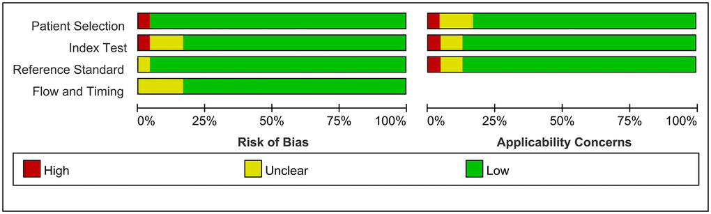
Figure 2. Risk of Bias and applicability concerns graph: Judgments about each domain presented as percentages across included studies.
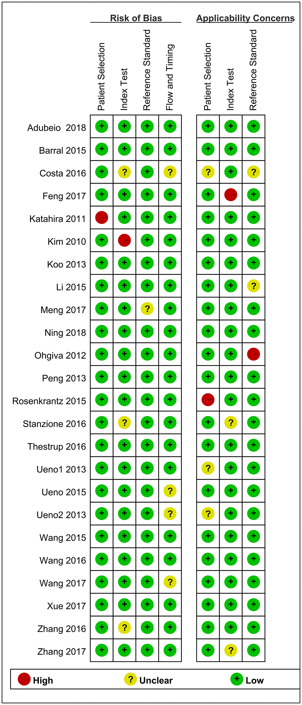
Figure 3. Risk of Bias and applicability concerns summary: judgments about each domain for each included study.
Pooling results
The Spearman correlation indicated no threshold effect (r = 0.317, P = 0.094). From the data obtained, we determined pooled sensitivity and specificity values of 0.84 (95% CI: 0.80–0.87) and 0.87 (95% CI: 0.81–0.91), respectively (Figure 4 and Figure 5). The AUC was 0.941(0.88–0.93) (Figure 6). The PLR and NLR were 6.4 (95% CI: 4.4–9.3, Supplementary Materials 2 and 3) and 0.19 (95% CI: 0.16–0.23), respectively, and the DOR was 34 (95% CI: 22 to 51, Supplementary Material 4). According to Fagan's nomogram (Figure 7), when the pretest probability was 20%, the corresponding post-test probability was 61% using the PLR and 5% using the NLR. The diagnostic performance was visualized by a likelihood ratio scattergram (Figure 8). All of these results suggest that the degree of diagnostic accuracy of high b-value DWI for detecting prostate cancer was relatively high.
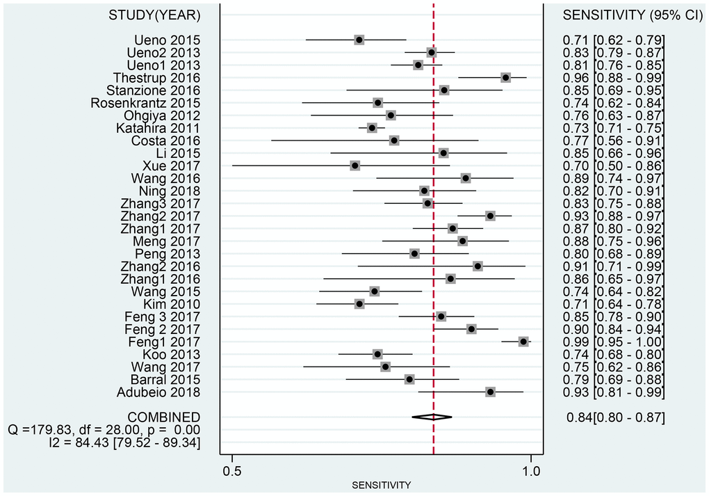
Figure 4. Forest plot of pooled sensitivity of diagnostic accuracy of high b-value DWI for detecting prostate cancer.
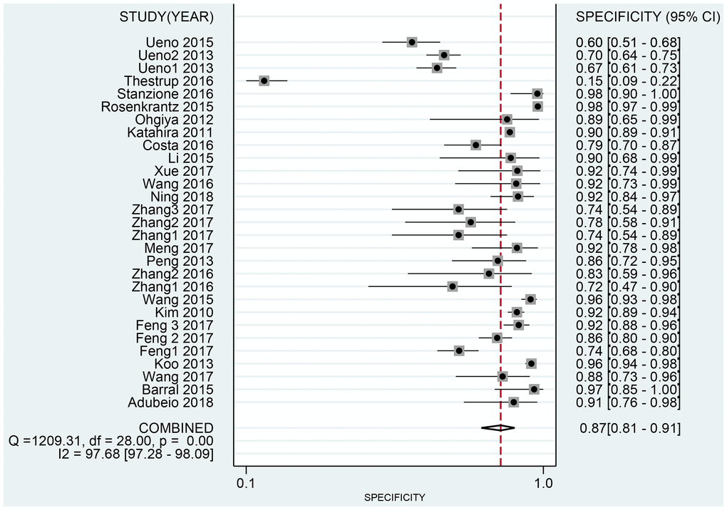
Figure 5. Forest plot of pooled specificity of diagnostic accuracy of high b-value DWI for detecting prostate cancer.
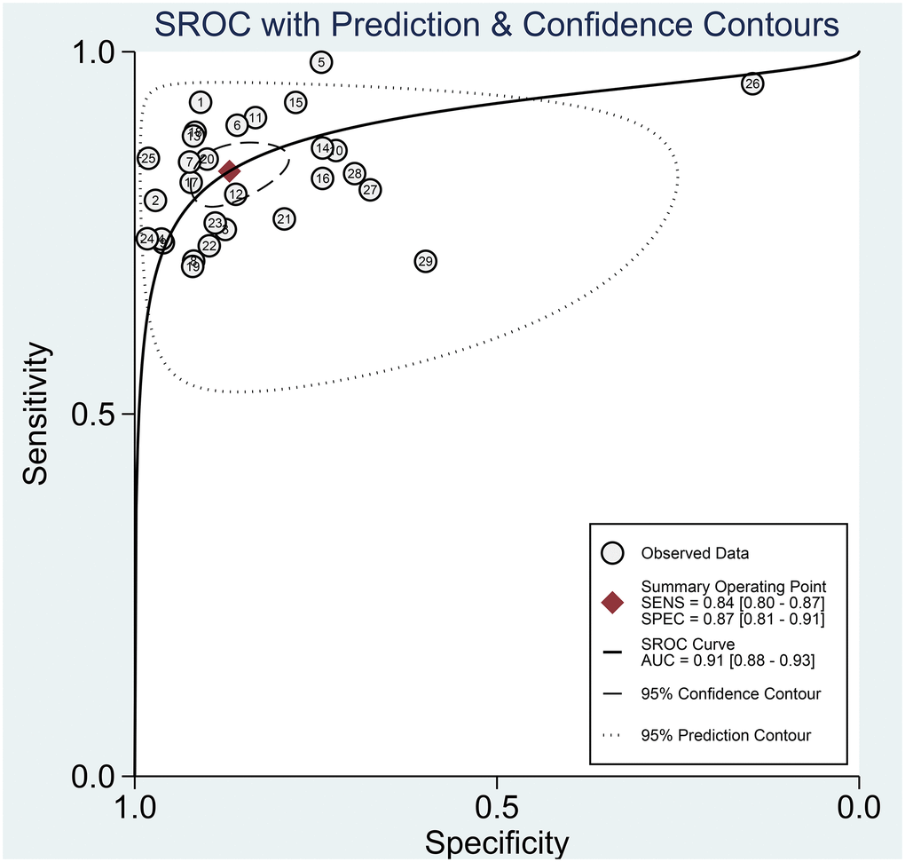
Figure 6. The SROC curve of diagnostic accuracy of high b-value DWI for detecting prostate cancer.
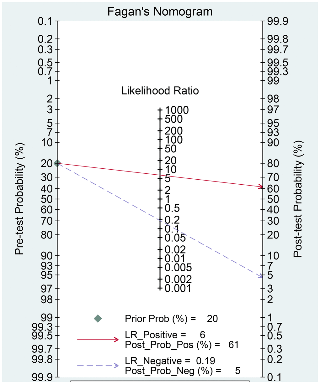
Figure 7. Fagan diagram evaluating the overall diagnostic value of high b-value for detecting prostate cancer.
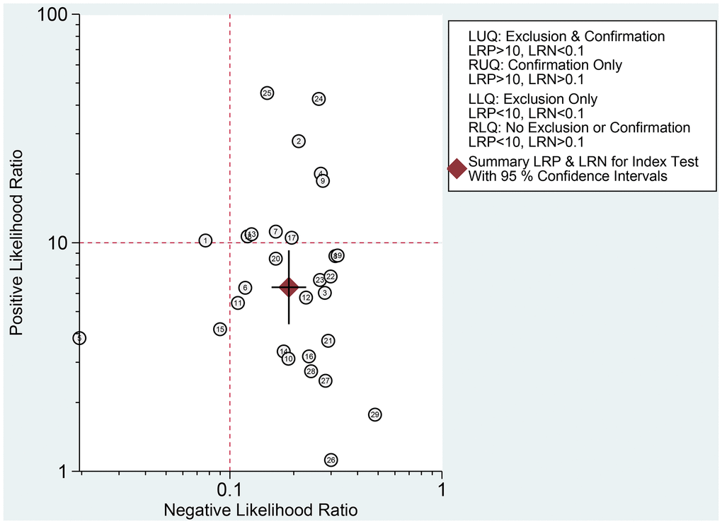
Figure 8. Likelihood ratio scatter gram.
Subgroup analysis
We conducted subgroup analyses of six subgroups (study design, number of patients, mean age of the patients, MRI field intensity, b-value, and DWI diagnostic measures) to identify the sources of heterogeneity. All results are shown in Table 4. The study design was divided into prospective and retrospective studies, and the sensitivity, specificity, PLR, NLR, and DOR showed no significant differences, but the AUC was significantly different, suggesting that it was a cause of the heterogeneity. The sensitivity, specificity, PLR, DOR, and AUC values were slightly superior for > 50 patients than for ≤ 50 patients, and the same trend was observed between those aged > 65 years and those aged ≤ 65 years. However, neither the number of patients nor the mean age showed a significant difference, suggesting that they did not contribute to the heterogeneity. MRI field intensity was divided into 1.5 T and 3.0 T, and the integrated sensitivity, specificity, PLR, NLR, DOR, and AUC values were 0.84, 0.83, 4.9, 0.19, 25, and 0.90 for 1.5T and 0.84, 0.88, 7.0, 0.19, 37, and 0.91 for 3.0T, respectively. There were no significant differences in any of these values between the two field intensities, suggesting that MRI field intensity did not contribute to the heterogeneity. Regarding b-values, the sensitivity, specificity, PLR, NLR, DOR, and AUC values were 0.83, 0.87, 6.6, 0.20, 33, and 0.90 for high b-values and 0.88, 0.86, 6.2, 0.14, 45, and 0.93 for ultrahigh b-values, respectively. Regarding DWI diagnostic measures, the sensitivity, specificity, PLR, NLR, DOR, and AUC values for ADC (quantitative) values were 0.89, 0.88, 7.6, 0.13, 58, and 0.94, and those for visual evaluation (qualitative) were 0.82, 0.86, 6.0, 0.21, 29, and 0.88. The results showed no significant differences between groups. Similar results were also found among different biopsy type, methods for identifying b-value. However, MRI supplier from Siemens and Ge seems to be prior to Philips (Philips: AUC (0.85, 95% CI: 0.82–0.88); Siemens: AUC (0.90, 95% CI: 0.88–0.83); Ge: AUC (0.94, 95% CI (0.91–0.96)) (Table 4). The heterogeneity was high within studies. The meta-regression indicated that publication year and population setting may cause the heterogeneity within studies (Table 5).
Table 4. Summary of pooled results.
| Subgroup | Sensitivity (95% CI) | Specificity (95% CI) | PLR (95% CI) | NLR (95% CI) | DOR (95% CI) | AUC (95% CI) |
| All studies | 0.84 (0.80–0.87) | 0.87 (0.81–0.91) | 6.4 (4.4–9.3) | 0.19 (0.16–0.23) | 34 (22–51) | 0.91 (0.88–0.93) |
| Study design | ||||||
| Prospective | 0.87 (0.82–0.90) | 0.90 (0.86–0.93) | 8.6 (6.4–11.6) | 0.15 (0.11–0.20) | 58 (44–78) | 0.95 (0.92–0.96) |
| Retrospective | 0.81 (0.76–0.85) | 0.83 (0.69–0.91) | 4.6 (2.6–8.2) | 0.23 (0.19–0.28) | 20 (11–36) | 0.86 (0.83–0.89) |
| Patients | ||||||
| ≤ 50 | 0.79 (0.73–0.84) | 0.86 (0.79–0.92) | 5.8 (3.6–9.5) | 0.23 (0.18–0.32) | 24 (12–48) | 0.87 (0.84–0.90) |
| > 50 | 0.85 (0.80–0.88) | 0.87 (0.79–0.93) | 6.6 (4.0–10.8) | 0.18 (0.14–0.22) | 37 (23–61) | 0.91 (0.88–0.93) |
| Mean age | ||||||
| ≤ 65 | 0.84 (0.80–0.88) | 0.87 (0.80–0.92) | 6.6 (4.3–10.1) | 0.18 (0.14–0.23) | 37 (23–60) | 0.92 (0.89–0.94) |
| > 65 | 0.83 (0.78–0.88) | 0.88 (0.83–0.92) | 6.8 (4.8–9.7) | 0.19 (0.15–0.25) | 36 (24–55) | 0.92 (0.89–0.94) |
| Field intensity | ||||||
| 1.5T | 0.84 (0.77–0.89) | 0.83 (0.75–0.89) | 4.9 (3.3–7.1) | 0.19 (0.14–0.27) | 25 (17–38) | 0.90 (0.87–0.93) |
| 3.0T | 0.84 (0.79–0.87) | 0.88 (0.81–0.93) | 7.0 (4.4–10.9) | 0.19 (0.15–0.23) | 37 (23–61) | 0.91 (0.88–0.93) |
| B–value | ||||||
| High | 0.83 (0.78–0.86) | 0.87 (0.80–0.92) | 6.6 (4.1–10.5) | 0.20 (0.16–0.24) | 33 (20–55) | 0.90 (0.87–0.92) |
| Ultra–high | 0.88 (0.84–0.92) | 0.86 (0.78–0.91) | 6.2 (4.0–9.5) | 0.14 (0.10–0.19) | 45 (26–78) | 0.93 (0.91–0.95) |
| DWI diagnostic measure | ||||||
| ADC value | 0.89 (0.79–0.94) | 0.88 (0.82–0.92) | 7.6 (5.3–10.9) | 0.13 (0.07–0.24) | 58 (36–94) | 0.94 (0.92–0.96) |
| Visual evaluation | 0.82 (0.78–0.85) | 0.86 (0.78–0.92) | 6.0 (3.7–9.7) | 0.21 (0.18–0.25) | 29 (17–49) | 0.88 (0.75–0.91) |
| Population setting | ||||||
| PCa | 0.84 (0.80–0.87) | 0.86 (0.80–0.91) | 6.2 (4.1–9.3) | 0.19 (0.16–0.23) | 33 (21–51) | 0.90 (0.87–0.93) |
| Biopsy type | ||||||
| Prostatectomy | 0.79 (0.75–0.83) | 0.87 (0.76–0.94) | 6.2 (3.3–11.7) | 0.24 (0.20–0.28) | 26 (13–51) | 0.85 (0.82–0.88) |
| Systematic biopsy | 0.87 (0.82–0.90) | 0.83 (0.76–0.88) | 5.1 (3.6–7.2) | 0.16 (0.12–0.22) | 32 (19–53) | 0.92 (0.89–0.94) |
| Targeted biopsy | 0.89 (0.78–0.95) | 0.88 (0.81–0.93) | 7.5 (5.1–11.0) | 0.12 (0.06–0.25) | 61 (36–101) | 0.94 (0.92–0.96) |
| Methods for identifying b–value | ||||||
| Signal extrapolation | 0.89 (0.81–0.94) | 0.87 (0.82–0.90) | 6.8 (5.2–8.7) | 0.12 (0.07–0.21) | 55 (35–87) | 0.93 (0.91–0.95) |
| Motion probing gradients | 0.82 (0.78–0.85) | 0.87 (0.78–0.93) | 6.3 (3.7–10.7) | 0.21 (0.18–0.25) | 30 (17–53) | 0.88 (0.84–0.90) |
Table 5. Meta-regression for heterogeneity within studies.
| Parameter | Estimate (95% CI) | P |
| Year of publication | 81.41 (60.32–100.00) | 0.00 |
| Age | 0.00 (0.00–100.00) | 0.44 |
| Sample size | 0.00 (0.00–100.00) | 0.71 |
| Field intensity | 0.00 (0.00–100.00) | 0.57 |
| DWI diagnostic measure | 0.00 (0.00–100.00) | 0.82 |
| Population setting | 62.30 (15.03–100.00) | 0.07 |
| Biopsy type | 41.73 (0.00–100.00) | 0.18 |
| Methods for identifying b value | 0.00 (0.00–100.00) | 0.86 |
Sensitivity analysis and publication bias
The sensitivity analysis is presented in Figure 9. The goodness of fit (A) and bivariate normality (B) show the degree of fitting of the regression line to the observed value. As shown, the observed value is distributed around the reference line. The observed values are stable. The influence analysis indicated that four studies may overestimate the pooled results. The outlier detection test indicated that two studies were out of the detection range. After excluding these studies, the pooled sensitivity, specificity did not change (results not show). In addition, we constructed Deek's plot, which indicated that there was no publication bias (t = −1.21, p = 0.240) (Figure 10).
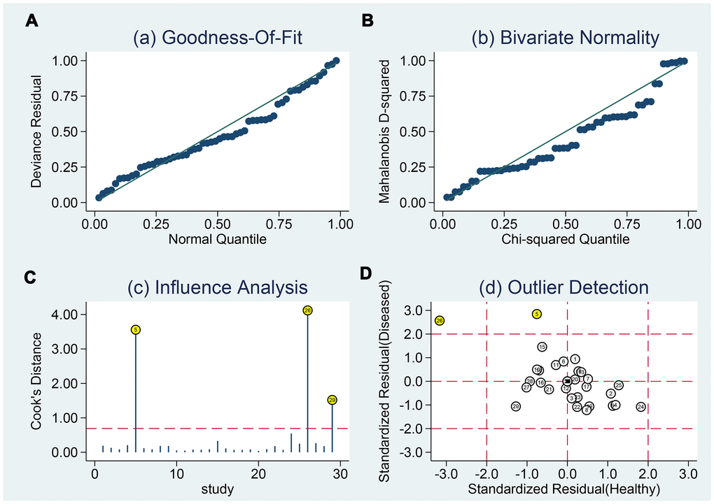
Figure 9. Sensitivity analyses. Graphical depiction of residual based goodness-of-fit (A), Bivariate normality (B), and influence (C) and outlier detection (D) analyses.
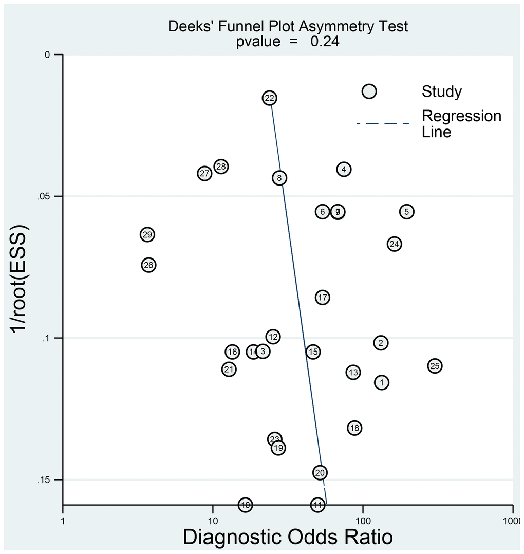
Figure 10. Deeks' funnel plot to evaluate the publication bias.
Discussion
This meta-analysis compared twenty-four studies evaluating the use of high b-value DWI to diagnose prostate cancer. Importantly, the analysis indicated that high b-value DWI had a high diagnostic accuracy with a high sensitivity (0.85; 95% CI: 0.81–0.88), specificity (0.89; 95% CI: 0.86–0.92), and AUC (0.94; 95% CI: 0.91–0.96). Based on these results, high b-value DWI can be used to detect prostate cancer in clinical practice.
DWI is crucial for diagnosing prostate cancer when using MRI. Compared with central lesions, peripheral lesions are easier to assess using DWI, which is consistent with the Prostate Imaging Reporting and Data System version 2 scoring system. The human prostate is a highly heterogeneous organ at the cellular level, and structural tissues show changes during the early stages on a scale of micrometers or smaller for many prostate pathologies. The ability of DWI to detect prostate cancer relies on the shrinkage of glands, tight cell arrangement, and increased parenchyma density, such that water diffuses slower in prostate cancer tissues than in normal prostate tissues [33–35], [37–39]. The b-value, which needs to be selected carefully in clinical applications, is a key parameter reflecting the sensitivity of DWI for detecting diffusional movements. A high b-value can better distinguish cancerous tissues from normal tissues; however, it also has some disadvantages, such as reducing the image signal-to-noise ratio, which obscures cancerous tissues [36]. But it is reported that Siemens developed Readout Segmentation of Long Variable Echo-trains DWI technology that adopts multiple excitation segmental readout for acquisition and K space filling, which significantly shortens echo time, reduces echo interval and improves image quality on DWI. The special targeting uniformity technology can also obtain the best magnetic field uniformity, further improve the magnetic field uniformity of complex parts, so as to further improve the image quality of DWI. This technology has been confirmed in several tumors [37–39].
There is no accepted standard range of b-values for DWI that is optimal for diagnosing prostate cancer.
Our results suggest that a high b-value is a robust tool for prostate cancer diagnosis. The high AUC (0.94; 95% CI: 0.91–0.96) together with the high pooled sensitivity (0.85; 95% CI: 0.81–0.88) and specificity (0.89; 95% CI: 0.86–0.92) signified its very good diagnostic accuracy. The PLR and NLR were 8.0 (95% CI: 6.2–10.4) and 0.17 (95% CI: 0.13–0.21), respectively. The former indicates that the rate of diagnosing prostate cancer using high b-value DWI is 8.0 times higher in prostate cancer patients than in patients without prostate cancer. The latter suggests that the possibility of high b-value DWI diagnosis not detecting prostate cancer in individuals with prostate cancer is 17%. That means a high possibility of prostate cancer exclusion. Therefore, high b-value DWI showed better diagnostic accuracy. In the present study, b values of all studies included in the meta-analysis are 2000s/mm2 or more, and We will recommend b value ≥ 2000s/mm2 as optimal standard for diagnosing PCa.
Although our study was carefully conducted, some issues were inevitable. To demonstrate the source of heterogeneity, we performed several subgroup analyses. The subgroups assessed in our study were study design, number of patients, mean age of the patients, MRI field intensity, b-values, and DWI diagnostic measures. Regarding study design, the sensitivity of the prospective studies was superior to that of the retrospective studies, despite no obvious differences between the two designs. Furthermore, the DOR was higher for the prospective studies than the retrospective studies, and the AUC showed a significant difference between the two groups. We therefore concluded that the study design was a source of the heterogeneity observed. MRI field intensity showed the most striking results in that the PLR and DOR were almost twice as high for the studies using 3.0 T than for those using 1.5 T, and the AUC showed a significant difference between the two groups. The MRI field intensity contributed more to the heterogeneity among studies than did the study design. The sensitivity of studies involving high b-values (2,000 s/mm2) was slightly lower and the specificity was slightly higher than that of studies involving ultrahigh b-values (> 2,000 s/mm2), and the DOR and AUC between the two groups showed no significant differences. With respect to the number of patients, the studies with > 50 patients (compared with ≤ 50 patients) showed a higher sensitivity, PLR, DOR, and AUC. The mean ages of the patients showed the same results as those for the number of patients, but the difference was not significant.
We also performed subgroup analysis for qualitative and quantitative evaluation, and the studies based on ADC values (quantitative) versus visual evaluation (qualitative) showed no differences, suggesting that they had little or no contribution to the heterogeneity among studies. Although visual evaluation relies on the experience and skills of the performer, it results in no overall changes. Although the diagnostic accuracy was almost indifferent, there were still differences in imaging characteristics. A previous study found that the image deformation of DWI is smaller, the lesion contrast is higher in qualitative analysis, and the ADC value of DWI sequences shows better repeatability in quantitative analysis than standard DWI sequences [40]. The Prostate Imaging Reporting and Data System version 2.1 has recommended qualitative evaluation of DWI [41].
There were some limitations for this study. (1) The heterogeneity was high within studies. Even when we conducted subgroup analyses, the heterogeneity was carefully considered. The meta-regression indicated that the year of publication and population setting can affect the estimations. Besides, human prostate cancer cells are heterogenous, containing a variety of cancer cells with phenotypical and functional discrepancies, and this may generate heterogeneity. However, almost none of studies provided prostate cancer cell types, all studies just distinguish PCa from the tissues. Further research was required.
(2) The prostate cancer stage of the patients in the selected studies was not clear, which may have influenced the diagnostic accuracies. (3) The language of the searched studies was restricted to English and Chinese, which may have reduced the representativeness of the included studies. (4) It is needless to say that repeatability of DWI signal decay derived parameters needs to be evaluated because high repeatability of measurements is a prerequisite for quantitative patient tailored treatment planning and therapy monitoring. Previous studies found that Monoexponential model demonstrated the highest repeatability and clinical values in the regions - of interest-based analysis of prostate cancer DWI. However, included studies did not introduce used modeling and this study was based on the b values in the range of 0–500/mm2. Modeling evaluation based on high b-values are required [42].
In summary, high b-value DWI showed high diagnostic accuracy in the qualitative and quantitative evaluation of prostate cancer. We should consider the possibility of its clinical application, although studies with large sample sizes and higher quality are needed, particularly for quantitative evaluation. In addition, publication bias should be carefully considered when interpreting and applying our results.
Methods
This meta-analysis was performed and reported according to the Preferred Reporting Items for Systematic Reviews and Meta-Analyses (PRISMA) guidelines listed in the PRISMA statement [43]. The PRISMA statement is provided in Supplementary Material 5.
Literature search
A comprehensive systematic literature search in the PubMed, Excerpta Medica Database (EMBASE), Cochrane Library, China National Knowledge Infrastructure, China Biology Medicine disc, and Wanfang databases was conducted to identify studies investigating the diagnostic performance of high b-value DWI for detecting prostate cancer. The search query combined synonyms and related terms of prostate cancer (“prostate disease,” “prostate tumor,” “prostate lesions,” and “PCa”), high b-value (“strong b-value,” “multiple b-value,” and “ultra-high b-value”), DWI, and diagnostic accuracy (“diagnostic performance,” “sensitivity,” “specificity,” and “receiver operator characteristic curve”). Logical operators (AND, NOT, and OR) were then used to conduct comprehensive combinations of these terms. The details of search strategy were provided in the Supplementary Material 6. Studies were restricted to English and Chinese languages, and the time span of the studies was January 1, 1995, to April 30, 2021. The references included in the identified papers were also screened to expand the range of our search.
Selection criteria
Two reviewers (LC and LN) independently conducted the study selection. Controversies were settled by discussion. Only studies that met all of the following criteria were chosen: (1) a retrospective or prospective design was used; (2) the purpose of the study was to evaluate the diagnostic value of high b-value DWI in prostate cancer alone or data for assessing accuracy of high b value for prostate cancer can be extracted. (3) the study used b-values ≥ 2000 s/mm2; (4) the study included ≥ 30 patients; (5) histopathological results (as the gold standard) were available for all patients; and (6) sufficient information was provided to establish 2 × 2 contingency tables and to calculate the sensitivity and specificity for detecting prostate cancer. Studies were excluded if they satisfied any of the following criteria: (1) reviews, case reports, dissertations, or unpublished articles; (2) inclusion of animal experimental data; and (3) combination with other MRI modalities (T2-weighted or dynamic contrast-enhanced imaging) to evaluate the diagnostic performance of high b-value DWI for prostate cancer.
Data extraction
One reviewer independently collected the data from the included studies using normative tables. The other reviewer double-checked this process. The following information was collected from the studies: author(s), country, study design, numbers of patients and lesions, mean age of the patients, PSA level range, MRI field intensity, MRI supplier, coil type, b-value, DWI diagnostic measures, population setting, biopsy type, diffusion times, DWI postprocessing, evaluation type (quantitively or qualitive), and methods for identifying the b-value. In addition, the numbers of TP (true positive), TN (true negative), FN (false negative) and FP (false positive) cases were collected to calculate the sensitivity and specificity. Disagreements in the data extraction findings were resolved via discussion or adjudication with a third reviewer.
Quality evaluation
Each paper’s quality was assessed using the Quality Assessment of Diagnostic Accuracy Studies 2, a validated tool specifically designed to evaluate diagnostic accuracy studies via four domains: flow and timing, patient selection, index test, and reference standard. A risk of bias existed in all four domains, but applicability concerns existed in only the last three domains. Both risk of bias and applicability concerns were graded as low, unclear, or high [44]. This step was conducted independently by two reviewers, and controversies were settled by discussion or by consulting a third party.
Statistical analysis
Using uses an exact binomial rendition of the bivariate mixed-effects regression model developed by von Houwelingen for treatment trial meta-analysis and modified for synthesis of diagnostic test data [45]. The pooled sensitivity, specificity, positive likelihood ratio (PLR), negative likelihood ratio (NLR), diagnostic odds ratio (DOR), and area under the SROC curve (AUC) along with 95% confidence intervals (CIs) were determined using Stata 14.0 software (https://www.stata.com/). The heterogeneity among studies was quantified using the Q test and I2 statistic [46]. The Q test was defined by Cochran and is calculated by summing the squared deviations of each study’s effect estimate from the overall effect estimate, weighting the contribution of each study by its inverse variance. The I2 index measures the extent of true heterogeneity, dividing the difference between the result of the Q test and its degrees of freedom by the Q value itself and multiplying by 100 [43]. An I2 > 50% and P < 0.05 were considered to indicate heterogeneity. Subgroup analysis was used to evaluate the heterogeneity among groups. The study design, number of patients, mean age of the patients, MRI field intensity, DWI diagnostic measures, and b-value were compared by subgroup analyses. The aim of our study was to understand the effect of high b-values and standard b-values on the diagnostic accuracy of prostate cancer, but without further analyses of the effect between high b-values and ultrahigh b-values, subgroup analyses were conducted. The concrete comparisons were (1) study design: prospective versus retrospective; (2) number of patients: ≤ 50 versus > 50; (3) mean age: ≤ 65 years versus > 65 years; (4) MRI field intensity: 1.5 T versus 3 T; (5) b-value: high (2,000) versus ultrahigh (> 2,000); and (6) DWI diagnostic measure: ADC values versus visual evaluations. Fagan’s nomogram was used to show the relevance of the prior test probability, likelihood ratio, and posterior test probability. Publication bias was visualized using Deek’s funnel plot. Meta-regression was performed for exploring the heterogeneity within studies. All statistical computations were conducted using Stata 14.0 software (Stata Corp, College Station, TX, USA), and the results were considered significant at P < 0.05.
Data availability
All data was within the manuscript without any restriction.
Supplementary Materials
Author Contributions
LC contributed this idea for the present study. SLF designed the search strategy. LN and LZZ extracted and collected data. LZZ provided analysis software. LC drafted the manuscript. LZZ revised this manuscript. All authors reviewed this manuscript and approved this submission.
Conflicts of Interest
The authors declare no conflicts of interest related to this study.
Funding
This work was partly supported by the Science Foundation of Xiangya Hospital for Young Scholar (ZL: NO. 2018Q012), National Natural Science Foundation of China (ZL: No. 82003239), and Hunan Province Natural Science Foundation (Youth Foundation Project) (ZL: NO. 2019JJ50945).
References
- 1. Jemal A, Center MM, DeSantis C, Ward EM. Global patterns of cancer incidence and mortality rates and trends. Cancer Epidemiol Biomarkers Prev. 2010; 19:1893–907. https://doi.org/10.1158/1055-9965.EPI-10-0437 [PubMed]
- 2. Lippi G, Montagnana M, Guidi GC, Plebani M. Prostate-specific antigen-based screening for prostate cancer in the third millennium: useful or hype? Ann Med. 2009; 41:480–89. https://doi.org/10.1080/07853890903156468 [PubMed]
- 3. Lin K, Croswell JM, Koenig H, Lam C, Maltz A. Prostate-Specific Antigen-Based Screening for Prostate Cancer: An Evidence Update for the U.S. Preventive Services Task Force. Rockville (MD): Agency for Healthcare Research and Quality (US); 2011 . Report No: 12-05160-EF-1. [PubMed]
- 4. Hayes JH, Barry MJ. Screening for prostate cancer with the prostate-specific antigen test: a review of current evidence. JAMA. 2014; 311:1143–49. https://doi.org/10.1001/jama.2014.2085 [PubMed]
- 5. Ahmed HU, El-Shater Bosaily A, Brown LC, Gabe R, Kaplan R, Parmar MK, Collaco-Moraes Y, Ward K, Hindley RG, Freeman A, Kirkham AP, Oldroyd R, Parker C, Emberton M, and PROMIS study group. Diagnostic accuracy of multi-parametric MRI and TRUS biopsy in prostate cancer (PROMIS): a paired validating confirmatory study. Lancet. 2017; 389:815–22. https://doi.org/10.1016/S0140-6736(16)32401-1 [PubMed]
- 6. Bammer R. Basic principles of diffusion-weighted imaging. Eur J Radiol. 2003; 45:169–84. https://doi.org/10.1016/s0720-048x(02)00303-0 [PubMed]
- 7. Weinreb JC, Barentsz JO, Choyke PL, Cornud F, Haider MA, Macura KJ, Margolis D, Schnall MD, Shtern F, Tempany CM, Thoeny HC, Verma S. PI-RADS Prostate Imaging - Reporting and Data System: 2015, Version 2. Eur Urol. 2016; 69:16–40. https://doi.org/10.1016/j.eururo.2015.08.052 [PubMed]
- 8. Barentsz JO, Richenberg J, Clements R, Choyke P, Verma S, Villeirs G, Rouviere O, Logager V, Fütterer JJ, and European Society of Urogenital Radiology. ESUR prostate MR guidelines 2012. Eur Radiol. 2012; 22:746–57. https://doi.org/10.1007/s00330-011-2377-y [PubMed]
- 9. Adubeiro N, Nogueira ML, Nunes RG, Ferreira HA, Ribeiro E, La Fuente JMF. Apparent diffusion coefficient in the analysis of prostate cancer: determination of optimal b-value pair to differentiate normal from malignant tissue. Clin Imaging. 2018; 47:90–95. https://doi.org/10.1016/j.clinimag.2017.09.004 [PubMed]
- 10. Barral M, Cornud F, Neuzillet Y, Lonchampt E, Lassalle L, Delonchamp NB, Scherrer A. Characteristics of undetected prostate cancer on diffusion-weighted MR Imaging at 3-Tesla with a b-value of 2000s/mm(2): Imaging-pathologic correlation. Diagn Interv Imaging. 2015; 96:923–29. https://doi.org/10.1016/j.diii.2015.03.004 [PubMed]
- 11. Wang X, Meng X, Fei F, Jiang Q. Diagnostic value of high b-value diffusion-weighted imaging in prostate cancer. 2017; 2354–56. http://en.cnki.com.cn/Article_en/CJFDTOTAL-XYXZ201712026.htm.
- 12. Li X, Zeng X, Jiang R. Diagnostic value of high b-value DWI relative signal intensity in prostate cancer. Chin J Biomed Eng. 2015; 21:533–37. https://doi.org/10.3760/cma.j.issn.1674-1927.2015.06.012
- 13. Koo JH, Kim CK, Choi D, Park BK, Kwon GY, Kim B. Response. Korean J Radiol. 2013; 14:866–67. [PubMed]
- 14. Feng Z, Min X, Margolis DJ, Duan C, Chen Y, Sah VK, Chaudhary N, Li B, Ke Z, Zhang P, Wang L. Evaluation of different mathematical models and different b-value ranges of diffusion-weighted imaging in peripheral zone prostate cancer detection using b-value up to 4500 s/mm2. PLoS One. 2017; 12:e0172127. https://doi.org/10.1371/journal.pone.0172127 [PubMed]
- 15. Kim CK, Park BK, Kim B. Diffusion-weighted MRI at 3 T for the evaluation of prostate cancer. AJR Am J Roentgenol. 2010; 194:1461–69. https://doi.org/10.2214/AJR.09.3654 [PubMed]
- 16. Wang L, Qi Z, Gao J, Ban X, Shi X, Xu K. Investigations on B values in Diffusion-Weighted Imaging for Evaluation of Prostate Cancer at 3T. J HeBei North. 2015; 31:63–67.
- 17. Zhang K, Zhang X, Zhong Y, Ma L, Wang H, Zhang X. Preliminary investigation of diagnostic value of ultra-high b-value based diffusion-weighted imaging; in prostate central gland diagnosis. Chin J Radiol. 2016; 50:357–61. https://doi.org/10.3760/cma.j.issn.1005-1201.2016.05.009
- 18. Peng Y, Jiang Y, Yang C, Brown JB, Antic T, Sethi I, Schmid-Tannwald C, Giger ML, Eggener SE, Oto A. Quantitative analysis of multiparametric prostate MR images: differentiation between prostate cancer and normal tissue and correlation with Gleason score--a computer-aided diagnosis development study. Radiology. 2013; 267:787–96. https://doi.org/10.1148/radiol.13121454 [PubMed]
- 19. Meng Z, Guo C, Tan W. The application of ultra-high b value DWI in the differential diagnosis of benign and malignant nodules of the central part of the prostate gland. Imaging. 2017; 23:1929–31. https://doi.org/10.3760/cma.j.issn.1007-1245.2017.12.037
- 20. Zhang Y, Chen S, Liao W, Wen Z, Xu J, He X. The diagnostic value of 1.5T magnetic resonance multi b DWI signal intensity for prostate cancer. J Pract Med Imaging. 2017; 18:194–97. http://dx.chinadoi.cn/10.16106/j.cnki.cn14-1281/r.2017.03.004.
- 21. Ning P, Shi D, Sonn GA, Vasanawala SS, Loening AM, Ghanouni P, Obara P, Shin LK, Fan RE, Hargreaves BA, Daniel BL. The impact of computed high b-value images on the diagnostic accuracy of DWI for prostate cancer: A receiver operating characteristics analysis. Sci Rep. 2018; 8:3409. https://doi.org/10.1038/s41598-018-21523-6 [PubMed]
- 22. Wang C, Dong Y, Ding H. The value of MRI 3.0T with high b value of diffusion weighted imaging in the diagnosis of Prostate Cancer. Geriatr Health Care. 2016; 22:295–97. http://en.cnki.com.cn/Article_en/CJFDTOTAL-LYBJ201605010.htm.
- 23. Xue HL, Wang LW, Chen Q, Yin XD, Gao W, Zhou X. Value of of Different B Value of Diffusion-Weighted Imaging in the Diagnosis of Central Prostate Nodules. China Medical equipment. 2017; 32:71–73. https://doi.org/10.3969/j.issn.1674-1633.2017.11.017
- 24. Costa DN, Yuan Q, Xi Y, Rofsky NM, Lenkinski RE, Lotan Y, Roehrborn CG, Francis F, Travalini D, Pedrosa I. Comparison of prostate cancer detection at 3-T MRI with and without an endorectal coil: A prospective, paired-patient study. Urol Oncol. 2016; 34:255.e7-255.e13. https://doi.org/10.1016/j.urolonc.2016.02.009 [PubMed]
- 25. Katahira K, Takahara T, Kwee TC, Oda S, Suzuki Y, Morishita S, Kitani K, Hamada Y, Kitaoka M, Yamashita Y. Ultra-high-b-value diffusion-weighted MR imaging for the detection of prostate cancer: evaluation in 201 cases with histopathological correlation. Eur Radiol. 2011; 21:188–96. https://doi.org/10.1007/s00330-010-1883-7 [PubMed]
- 26. Ohgiya Y, Suyama J, Seino N, Hashizume T, Kawahara M, Sai S, Saiki M, Munechika J, Hirose M, Gokan T. Diagnostic accuracy of ultra-high-b-value 3.0-T diffusion-weighted MR imaging for detection of prostate cancer. Clin Imaging. 2012; 36:526–31. https://doi.org/10.1016/j.clinimag.2011.11.016 [PubMed]
- 27. Rosenkrantz AB, Kim S, Campbell N, Gaing B, Deng FM, Taneja SS. Transition zone prostate cancer: revisiting the role of multiparametric MRI at 3 T. AJR Am J Roentgenol. 2015; 204:W266–72. https://doi.org/10.2214/AJR.14.12955 [PubMed]
- 28. Stanzione A, Imbriaco M, Cocozza S, Fusco F, Rusconi G, Nappi C, Mirone V, Mangiapia F, Brunetti A, Ragozzino A, Longo N. Biparametric 3T Magnetic Resonance Imaging for prostatic cancer detection in a biopsy-naïve patient population: a further improvement of PI-RADS v2? Eur J Radiol. 2016; 85:2269–74. https://doi.org/10.1016/j.ejrad.2016.10.009 [PubMed]
- 29. Thestrup KC, Logager V, Baslev I, Møller JM, Hansen RH, Thomsen HS. Biparametric versus multiparametric MRI in the diagnosis of prostate cancer. Acta Radiol Open. 2016; 5:2058460116663046. https://doi.org/10.1177/2058460116663046 [PubMed]
- 30. Ueno Y, Kitajima K, Sugimura K, Kawakami F, Miyake H, Obara M, Takahashi S. Ultra-high b-value diffusion-weighted MRI for the detection of prostate cancer with 3-T MRI. J Magn Reson Imaging. 2013; 38:154–60. https://doi.org/10.1002/jmri.23953 [PubMed]
- 31. Ueno Y, Takahashi S, Kitajima K, Kimura T, Aoki I, Kawakami F, Miyake H, Ohno Y, Sugimura K. Computed diffusion-weighted imaging using 3-T magnetic resonance imaging for prostate cancer diagnosis. Eur Radiol. 2013; 23:3509–16. https://doi.org/10.1007/s00330-013-2958-z [PubMed]
- 32. Ueno Y, Takahashi S, Ohno Y, Kitajima K, Yui M, Kassai Y, Kawakami F, Miyake H, Sugimura K. Computed diffusion-weighted MRI for prostate cancer detection: the influence of the combinations of b-values. Br J Radiol. 2015; 88:20140738. https://doi.org/10.1259/bjr.20140738 [PubMed]
- 33. Lemberskiy G, Fieremans E, Veraart J, Deng FM, Rosenkrantz AB, Novikov DS. Characterization of prostate microstructure using water diffusion and NMR relaxation. Front Phys. 2018; 6:91. https://doi.org/10.3389/fphy.2018.00091 [PubMed]
- 34. Tong A, Lemberskiy G, Huang C, Shanbhogue K, Feiweier T, Rosenkrantz AB. Exploratory study of geometric distortion correction of prostate diffusion-weighted imaging using B0 map acquisition. J Magn Reson Imaging. 2019; 50:1614–19. https://doi.org/10.1002/jmri.26751 [PubMed]
- 35. Lemberskiy G, Rosenkrantz AB, Veraart J, Taneja SS, Novikov DS, Fieremans E. Time-Dependent Diffusion in Prostate Cancer. Invest Radiol. 2017; 52:405–11. https://doi.org/10.1097/RLI.0000000000000356 [PubMed]
- 36. Vallini V, Ortori S, Boraschi P, Manassero F, Gabelloni M, Faggioni L, Selli C, Bartolozzi C. Staging of pelvic lymph nodes in patients with prostate cancer: Usefulness of multiple b value SE-EPI diffusion-weighted imaging on a 3.0 T MR system. Eur J Radiol Open. 2015; 3:16–21. https://doi.org/10.1016/j.ejro.2015.11.004 [PubMed]
- 37. Tu C, Shen H, Liu D, Chen Q, Yuan X, Li X, Wang X, Liu R, Wang X, Li Q, Liu W, Zhang J. Simultaneous multi-slice readout-segmentation of long variable echo-trains for accelerated diffusion-weighted imaging of nasopharyngeal carcinoma: A feasibility and optimization study. Clin Imaging. 2021; 79:119–24. https://doi.org/10.1016/j.clinimag.2021.04.009 [PubMed]
- 38. Xie M, Ren Z, Bian D, Li D, Yu L, Zhu F, Huang R, Zhang Z, Suye S, Fu C. High resolution diffusion-weighted imaging with readout segmentation of long variable echo-trains for determining myometrial invasion in endometrial carcinoma. Cancer Imaging. 2020; 20:66. https://doi.org/10.1186/s40644-020-00346-7 [PubMed]
- 39. Zhang BT, Li M, Yu LL, Dai YM, Yu SN, Jiang JL. Diffusion tensor imaging of spinal microstructure in healthy adults: improved resolution with the readout segmentation of long variable echo-trains. Neural Regen Res. 2017; 12:2067–70. https://doi.org/10.4103/1673-5374.221166 [PubMed]
- 40. Wang Y, Lin Y, Zhou C, Zhang J, Zhang Z. Reduced field-of-view diffusion weighted imaging in diagnosis of prostate cancer. J Med Imaging. 2016; 29. http://en.cnki.com.cn/Article_en/CJFDTotal-JLYB201604014.htm.
- 41. Turkbey B, Rosenkrantz AB, Haider MA, Padhani AR, Villeirs G, Macura KJ, Tempany CM, Choyke PL, Cornud F, Margolis DJ, Thoeny HC, Verma S, Barentsz J, Weinreb JC. Prostate Imaging Reporting and Data System Version 2.1: 2019 Update of Prostate Imaging Reporting and Data System Version 2. Eur Urol. 2019; 76:340–51. https://doi.org/10.1016/j.eururo.2019.02.033
- 42. Merisaari H, Movahedi P, Perez IM, Toivonen J, Pesola M, Taimen P, Boström PJ, Pahikkala T, Kiviniemi A, Aronen HJ, Jambor I. Fitting methods for intravoxel incoherent motion imaging of prostate cancer on region of interest level: Repeatability and gleason score prediction. Magn Reson Med. 2017; 77:1249–64. https://doi.org/10.1002/mrm.26169 [PubMed]
- 43. Moher D, Liberati A, Tetzlaff J, Altman DG, and PRISMA Group. Preferred reporting items for systematic reviews and meta-analyses: the PRISMA statement. PLoS Med. 2009; 6:e1000097. https://doi.org/10.1371/journal.pmed.1000097 [PubMed]
- 44. Whiting PF, Rutjes AW, Westwood ME, Mallett S, Deeks JJ, Reitsma JB, Leeflang MM, Sterne JA, Bossuyt PM, and QUADAS-2 Group. QUADAS-2: a revised tool for the quality assessment of diagnostic accuracy studies. Ann Intern Med. 2011; 155:529–36. https://doi.org/10.7326/0003-4819-155-8-201110180-00009 [PubMed]
- 45. Chu H, Cole SR. Bivariate meta-analysis of sensitivity and specificity with sparse data: a generalized linear mixed model approach. J Clin Epidemiol. 2006; 59:1331–32. https://doi.org/10.1016/j.jclinepi.2006.06.011 [PubMed]
- 46. Biggerstaff BJ, Tweedie RL. Incorporating variability in estimates of heterogeneity in the random effects model in meta-analysis. Stat Med. 1997; 16:753–68. https://doi.org/10.1002/(sici)1097-0258(19970415)16:7<753::aid-sim494>3.0.co;2-g [PubMed]